В этом руководстве объясняется, как быстро начать отправлять запросы к REST API Earth Engine из Python с помощью Google Colab . Те же принципы применимы и к доступу к API из других языков и сред.
Примечание: REST API содержит новые и расширенные функции, которые могут быть неподходящими для всех пользователей. Если вы новичок в Earth Engine, ознакомьтесь с руководством по JavaScript .
 Просмотреть исходный код на GitHub
Прежде чем начать
Следуйте этим инструкциям , чтобы:
Настройте свой блокнот Colab
Если вы начинаете этот быстрый старт с нуля, вы можете создать новый блокнот Colab, нажав кнопку «Новый блокнот» на стартовой странице Colab и вставив приведенные ниже примеры кода в новую ячейку кода. В Colab уже установлен Cloud SDK . Он включает в себя инструмент командной строки gcloud , который можно использовать для управления облачными сервисами. Вы также можете запустить демонстрационный блокнот, нажав кнопку в начале этой страницы.
Аутентификация в Google Cloud
Первое, что нужно сделать, — это войти в систему, чтобы иметь возможность отправлять аутентифицированные запросы в Google Cloud.
В Colab вы можете запустить:
PROJECT = 'my-project'
!gcloud auth login --project {PROJECT}
(Или, если вы работаете локально, из командной строки, предполагая, что у вас установлен Cloud SDK:)
PROJECT='my-project'
gcloud auth login --project $PROJECT
Примите решение войти в систему, используя свою учетную запись Google, и завершите процесс входа.
Получите файл закрытого ключа для вашей учетной записи службы.
Прежде чем использовать учетную запись сервиса для аутентификации, необходимо загрузить файл закрытого ключа. Для этого в Colab выполните загрузку в виртуальную машину Notebook:
SERVICE_ACCOUNT='foo-name@project-name.iam.gserviceaccount.com'
KEY = 'my-secret-key.json'
!gcloud iam service-accounts keys create {KEY} --iam-account {SERVICE_ACCOUNT}
Или альтернативно из командной строки:
SERVICE_ACCOUNT='foo-name@project-name.iam.gserviceaccount.com'
KEY='my-secret-key.json'
gcloud iam service-accounts keys create $KEY --iam-account $SERVICE_ACCOUNT
Доступ к вашим учетным данным и их проверка
Теперь вы готовы отправить свой первый запрос к API Earth Engine. Используйте закрытый ключ для получения учётных данных. Используйте эти учётные данные для создания авторизованного сеанса для выполнения HTTP-запросов. Вы можете ввести их в новую ячейку кода в блокноте Colab. (Если вы используете командную строку, убедитесь, что установлены необходимые библиотеки).
from google.auth.transport.requests import AuthorizedSession
from google.oauth2 import service_account

credentials = service_account.Credentials.from_service_account_file(KEY)
scoped_credentials = credentials.with_scopes(
    ['https://www.googleapis.com/auth/cloud-platform'])

session = AuthorizedSession(scoped_credentials)

url = 'https://earthengine.googleapis.com/v1alpha/projects/earthengine-public/assets/LANDSAT'

response = session.get(url)

from pprint import pprint
import json
pprint(json.loads(response.content))
Если все настроено правильно, то запуск этой команды даст следующий вывод:
{'id': 'LANDSAT',
 'name': 'projects/earthengine-public/assets/LANDSAT',
 'type': 'FOLDER'}
Выберите набор данных
Вы можете искать и изучать доступные наборы данных с помощью редактора кода Earth Engine по адресу code.earthengine.google.com . Давайте найдём данные Sentinel 2. (Если вы впервые используете редактор кода, при входе в систему вам будет предложено разрешить доступ к Earth Engine от вашего имени.) В редакторе кода введите «sentinel» в поле поиска вверху. Появится несколько наборов растровых данных:
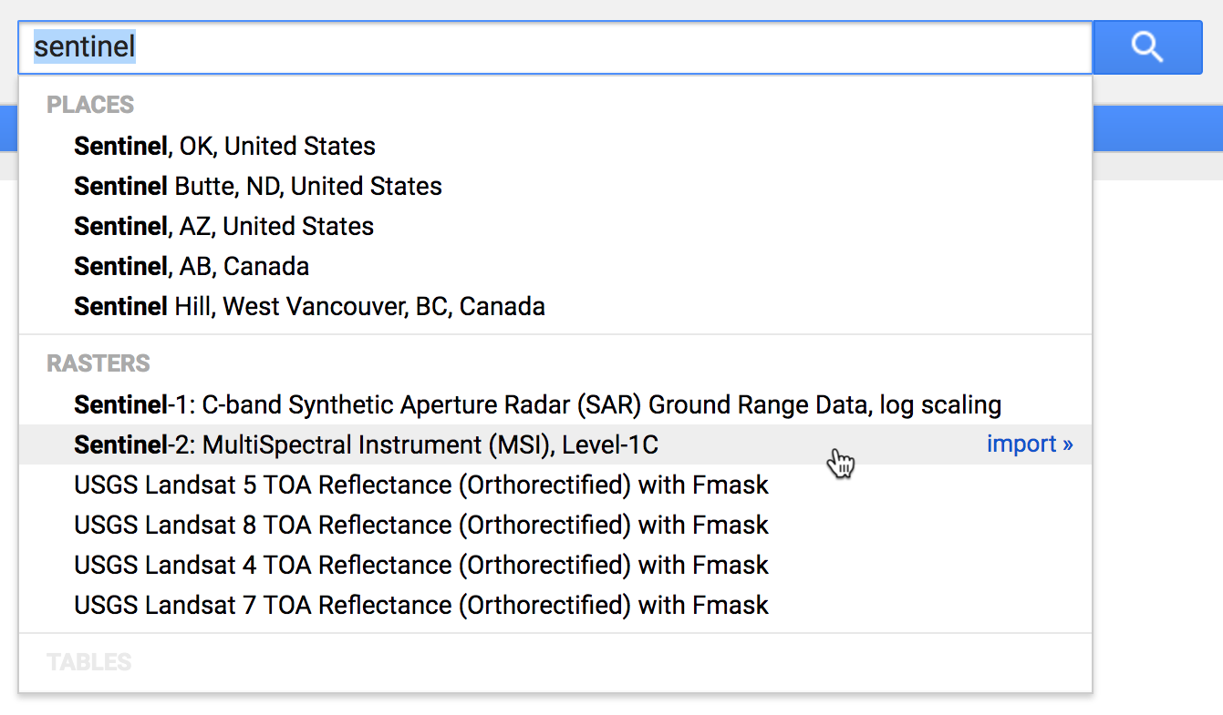
Нажмите на ссылку «Sentinel-2: Многоспектральный прибор (MSI), Уровень 1C»:
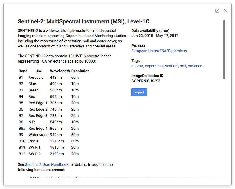
Страницы описания наборов данных, подобные этой, содержат важную информацию, необходимую для использования любого набора данных в каталоге открытых данных Earth Engine, включая краткое описание набора данных, ссылки на поставщика данных для получения дополнительных сведений, информацию о любых ограничениях использования, которые могут применяться к набору данных, а также идентификатор актива Earth Engine набора данных.
В этом случае мы видим в правой части окна, что это ресурс коллекции изображений, путь к которому — COPERNICUS/S2 .
Запрос определенных изображений
Этот набор данных Sentinel-2 включает более двух миллионов изображений, охватывающих весь мир с 2015 года по настоящее время. Давайте выполним запрос projects.assets.listImages к коллекции изображений, чтобы найти данные за апрель 2017 года с низкой облачностью, включая конкретную точку в Маунтин-Вью, Калифорния.
import urllib

coords = [-122.085, 37.422]

project = 'projects/earthengine-public'
asset_id = 'COPERNICUS/S2'
name = '{}/assets/{}'.format(project, asset_id)
url = 'https://earthengine.googleapis.com/v1alpha/{}:listImages?{}'.format(
  name, urllib.parse.urlencode({
    'startTime': '2017-04-01T00:00:00.000Z',
    'endTime': '2017-05-01T00:00:00.000Z',
    'region': '{"type":"Point", "coordinates":' + str(coords) + '}',
    'filter': 'CLOUDY_PIXEL_PERCENTAGE < 10',
}))

response = session.get(url)
content = response.content

for asset in json.loads(content)['images']:
    id = asset['id']
    cloud_cover = asset['properties']['CLOUDY_PIXEL_PERCENTAGE']
    print('%s : %s' % (id, cloud_cover))
Этот скрипт запрашивает коллекцию соответствующих изображений, декодирует полученный ответ JSON и выводит идентификатор объекта и облачность для каждого соответствующего изображения. Результат должен выглядеть следующим образом:
COPERNICUS/S2/20170420T184921_20170420T190203_T10SEG : 4.3166
COPERNICUS/S2/20170430T190351_20170430T190351_T10SEG : 0
Очевидно, над этой точкой имеются два снимка, сделанные в этом месяце, на которых запечатлена низкая облачность.
Осмотрите конкретное изображение
Похоже, что на одном из совпадающих объектов практически нет облачности. Давайте подробнее рассмотрим этот ресурс с идентификатором COPERNICUS/S2/20170430T190351_20170430T190351_T10SEG . Обратите внимание, что все ресурсы из публичного каталога принадлежат проекту earthengine-public . Вот фрагмент кода на Python, который выполнит запрос projects.assets.get для получения информации об этом ресурсе по идентификатору, выведет доступные диапазоны данных и более подробную информацию о первом диапазоне:
asset_id = 'COPERNICUS/S2/20170430T190351_20170430T190351_T10SEG'
name = '{}/assets/{}'.format(project, asset_id)
url = 'https://earthengine.googleapis.com/v1alpha/{}'.format(name)

response = session.get(url)
content = response.content

asset = json.loads(content)
print('Band Names: %s' % ','.join(band['id'] for band in asset['bands']))
print('First Band: %s' % json.dumps(asset['bands'][0], indent=2, sort_keys=True))
Вывод должен выглядеть примерно так:
Band Names: B1,B2,B3,B4,B5,B6,B7,B8,B8A,B9,B10,B11,B12,QA10,QA20,QA60
First Band: {
  "dataType": {
    "precision": "INTEGER",
    "range": {
      "max": 65535
    }
  },
  "grid": {
    "affineTransform": {
      "scaleX": 60,
      "scaleY": -60,
      "translateX": 499980,
      "translateY": 4200000
    },
    "crsCode": "EPSG:32610",
    "dimensions": {
      "height": 1830,
      "width": 1830
    }
  },
  "id": "B1",
  "pyramidingPolicy": "MEAN"
}
Список диапазонов данных соответствует тому, что мы видели ранее в описании набора данных . Мы видим, что этот набор данных содержит 16-битные целочисленные данные в системе координат EPSG:32610 , или зоне UTM 10N. Этот первый диапазон имеет идентификатор B1 и разрешение 60 метров на пиксель. Начало координат изображения находится в точке (499980,4200000) в этой системе координат.
Отрицательное значение affineTransform.scaleY указывает на то, что начало координат находится в северо-западном углу изображения, как это обычно и бывает: увеличение индексов пикселей y соответствует уменьшению пространственных координат y (направление на юг).
Получение значений пикселей
Давайте выполним запрос projects.assets.getPixels для извлечения данных из каналов высокого разрешения этого изображения. На странице описания набора данных указано, что каналы B2 , B3 , B4 и B8 имеют разрешение 10 метров на пиксель. Этот скрипт извлекает данные из верхнего левого угла размером 256x256 пикселей из этих четырёх каналов. Загрузка данных в формате numpy упрощает декодирование ответа в массив данных Python.
import numpy
import io

name = '{}/assets/{}'.format(project, asset_id)
url = 'https://earthengine.googleapis.com/v1alpha/{}:getPixels'.format(name)
body = json.dumps({
    'fileFormat': 'NPY',
    'bandIds': ['B2', 'B3', 'B4', 'B8'],
    'grid': {
        'affineTransform': {
            'scaleX': 10,
            'scaleY': -10,
            'translateX': 499980,
            'translateY': 4200000,
        },
        'dimensions': {'width': 256, 'height': 256},
    },
})

pixels_response = session.post(url, body)
pixels_content = pixels_response.content

array = numpy.load(io.BytesIO(pixels_content))
print('Shape: %s' % (array.shape,))
print('Data:')
print(array)
Вывод должен выглядеть так:
Shape: (256, 256)
Data:
[[( 899, 586, 351, 189) ( 918, 630, 501, 248) (1013, 773, 654, 378) ...,
  (1014, 690, 419, 323) ( 942, 657, 424, 260) ( 987, 691, 431, 315)]
 [( 902, 630, 541, 227) (1059, 866, 719, 429) (1195, 922, 626, 539) ...,
  ( 978, 659, 404, 287) ( 954, 672, 426, 279) ( 990, 678, 397, 304)]
 [(1050, 855, 721, 419) (1257, 977, 635, 569) (1137, 770, 400, 435) ...,
  ( 972, 674, 421, 312) (1001, 688, 431, 311) (1004, 659, 378, 284)]
 ...,
 [( 969, 672, 375, 275) ( 927, 680, 478, 294) (1018, 724, 455, 353) ...,
  ( 924, 659, 375, 232) ( 921, 664, 438, 273) ( 966, 737, 521, 306)]
 [( 920, 645, 391, 248) ( 979, 728, 481, 327) ( 997, 708, 425, 324) ...,
  ( 927, 673, 387, 243) ( 927, 688, 459, 284) ( 962, 732, 509, 331)]
 [( 978, 723, 449, 330) (1005, 712, 446, 314) ( 946, 667, 393, 269) ...,
  ( 949, 692, 413, 271) ( 927, 689, 472, 285) ( 966, 742, 516, 331)]]
Чтобы выбрать другой набор пикселей из этого изображения, просто укажите соответствующее значение affineTransform . Помните, что affineTransform задаётся в пространственной системе координат изображения; если вы хотите изменить положение начала координат в пиксельных координатах, используйте эту простую формулу:
request_origin = image_origin + pixel_scale * offset_in_pixels
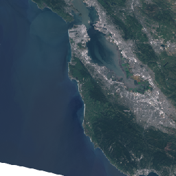
Создание миниатюрного изображения
Аналогичный механизм можно использовать для создания RGB-миниатюры этого изображения. Вместо запроса данных в исходном разрешении мы явно укажем область и размеры изображения. Чтобы получить миниатюру всего изображения, можно использовать геометрию контура изображения в качестве запрашиваемой области. Наконец, указав красный, зелёный и синий каналы изображения и соответствующий диапазон значений данных, мы можем получить привлекательную RGB-миниатюру.
Если собрать все это вместе, то фрагмент кода Python будет выглядеть следующим образом (с использованием виджета отображения изображений Colab IPython ):
url = 'https://earthengine.googleapis.com/v1alpha/{}:getPixels'.format(name)
body = json.dumps({
    'fileFormat': 'PNG',
    'bandIds': ['B4', 'B3', 'B2'],
    'region': asset['geometry'],
    'grid': {
        'dimensions': {'width': 256, 'height': 256},
    },
    'visualizationOptions': {
        'ranges': [{'min': 0, 'max': 3000}],
    },
})

image_response = session.post(url, body)
image_content = image_response.content

from IPython.display import Image
Image(image_content)
Вот получившееся уменьшенное изображение: