
Introduction
This document describes how to build a site selection solution by combining the Places Insights dataset, public geospatial data in BigQuery, and the Place Details API.
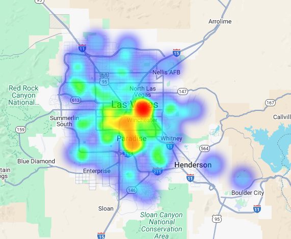
The map above illustrates the output of a demo given at Google Cloud Next 2025, which is available to watch on YouTube. You can run the code used to generate these results using the example notebook.
 View source on GitHub
The Business Challenge
Imagine you own a successful chain of coffee shops and want to expand into a new state, like Nevada, where you have no presence. Opening a new location is a significant investment, and making a data-driven decision is critical to success. Where do you even begin?
This guide walks you through a multi-layered analysis to pinpoint the optimal location for a new coffee shop. We'll start with a state-wide view, progressively narrow our search to a specific county and commercial zone, and finally perform a hyper-local analysis to score individual areas and identify market gaps by mapping out competitors.
Solution Workflow
This process follows a logical funnel, starting broad and getting progressively more granular to refine the search area and increase confidence in the final site selection.
Prerequisites and Environment Setup
Before diving into the analysis, you need an environment with a few key capabilities. While this guide will walk through an implementation using SQL and Python, the general principles can be applied to other technology stacks.
As a prerequisite, ensure your environment can:
- Execute queries in BigQuery.
- Access Places Insights, see Setup Places Insights for more information
- Subscribe to public datasets from
bigquery-public-dataand the US Census Bureau County Population Totals
You also need to be able to visualize geospatial data on a map, which is crucial for interpreting the results of each analytical step. There are many ways to achieve this. You could use BI tools like Looker Studio which connect directly to BigQuery, or you could use data science languages like Python.
State-Level Analysis: Find the Best County
Our first step is a broad analysis to identify the most promising county in Nevada. We'll define promising as a combination of high population and a high density of existing restaurants, which indicates a strong food and beverage culture.
Our BigQuery query accomplishes this by leveraging the built-in address
components available within the Places Insights dataset. The query counts
restaurants by first filtering the data to include only places within the state
of Nevada, using the administrative_area_level_1_name field. It then further
refines this set to include only places where the types array contains
'restaurant'. Finally, it groups these results by county name
(administrative_area_level_2_name) to produce a count for each county. This
approach utilizes the dataset's built-in, pre-indexed address structure.
This excerpt shows how we join county geometries with Places Insights and filter
for a specific place type, restaurant:
SELECT WITH AGGREGATION_THRESHOLD
  administrative_area_level_2_name,
  COUNT(*) AS restaurant_count
FROM
  `places_insights___us.places`
WHERE
  -- Filter for the state of Nevada
  administrative_area_level_1_name = 'Nevada'
  -- Filter for places that are restaurants
  AND 'restaurant' IN UNNEST(types)
  -- Filter for operational places only
  AND business_status = 'OPERATIONAL'
  -- Exclude rows where the county name is null
  AND administrative_area_level_2_name IS NOT NULL
GROUP BY
  administrative_area_level_2_name
ORDER BY
  restaurant_count DESC
A raw count of restaurants isn't enough; we need to balance it with population data to get a true sense of market saturation and opportunity. We will use population data from the US Census Bureau County Population Totals.
To compare these two very different metrics (a place count versus a large
population number), we use min-max normalization. This technique scales both
metrics to a common range (0 to 1). We then combine them into a single
normalized_score, giving each metric a 50% weight for a balanced comparison.
This excerpt shows the core logic for calculating the score. It combines normalized population and restaurant counts:
(
    -- Normalize restaurant count (scales to a 0-1 value) and apply 50% weight
    SAFE_DIVIDE(restaurant_count - min_restaurants, max_restaurants - min_restaurants) * 0.5
    +
    -- Normalize population (scales to a 0-1 value) and apply 50% weight
    SAFE_DIVIDE(population_2023 - min_pop, max_pop - min_pop) * 0.5
  ) AS normalized_score
After running the full query, a list of the counties, count of restaurants,
population, and normalized score is returned. Ordering by normalized_score
DESC reveals Clark County as the clear winner for further investigation as the
top contender.
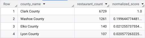
This screenshot shows the top 4 counties by normalized score. Raw population count has been purposefully omitted from this example.
County-Level Analysis: Find the Busiest Commercial Zones
Now that we've identified Clark County, the next step is to zoom in to find the ZIP codes with the highest commercial activity. Based on data from our existing coffee shops, we know that performance is better when located near a high density of major brands, so we'll use this as a proxy for high foot traffic.
This query uses the brands table within Places Insights, which contains
information about specific brands. This table can be
queried to discover the list of
supported brands. We first define a list of our target brands and then join this
with the main Places Insights dataset to count how many of these specific stores
fall within each ZIP code in Clark County.
The most efficient way to achieve this is with a two-step approach:
- First, we'll perform a fast, non-geospatial aggregation to count the brands within each postal code.
- Second, we'll join those results to a public dataset to get the map boundaries for visualization.
Count Brands Using the postal_code_names Field
This first query performs the core counting logic. It filters for places in
Clark County and then unnests the postal_code_names array to group the brand
counts by postal code.
WITH brand_names AS (
  -- First, select the chains we are interested in by name
  SELECT
    id,
    name
  FROM
    `places_insights___us.brands`
  WHERE
    name IN ('7-Eleven', 'CVS', 'Walgreens', 'Subway Restaurants', "McDonald's")
)
SELECT WITH AGGREGATION_THRESHOLD
  postal_code,
  COUNT(*) AS total_brand_count
FROM
  `places_insights___us.places` AS places_table,
  -- Unnest the built-in postal code and brand ID arrays
  UNNEST(places_table.postal_code_names) AS postal_code,
  UNNEST(places_table.brand_ids) AS brand_id
JOIN
  brand_names
  ON brand_names.id = brand_id
WHERE
  -- Filter directly on the administrative area fields in the places table
  places_table.administrative_area_level_2_name = 'Clark County'
  AND places_table.administrative_area_level_1_name = 'Nevada'
GROUP BY
  postal_code
ORDER BY
  total_brand_count DESC
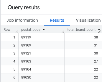
The output is a table of postal codes and their corresponding brand counts.
Attach ZIP Code Geometries for Mapping
Now that we have the counts, we can get the polygon shapes needed for
visualization. This second query takes our first query, wraps it in a Common
Table Expression (CTE) named brand_counts_by_zip, and joins its results to the
public geo_us_boundaries.zip_codes table. This efficiently attaches the
geometry to our pre-calculated counts.
WITH brand_counts_by_zip AS (
  -- This will be the entire query from the previous step, without the final ORDER BY (excluded for brevity).
  . . .
)
-- Now, join the aggregated results to the boundaries table
SELECT
  counts.postal_code,
  counts.total_brand_count,
  -- Simplify the geometry for faster rendering in maps
  ST_SIMPLIFY(zip_boundaries.zip_code_geom, 100) AS geography
FROM
  brand_counts_by_zip AS counts
JOIN
  `bigquery-public-data.geo_us_boundaries.zip_codes` AS zip_boundaries
  ON counts.postal_code = zip_boundaries.zip_code
ORDER BY
  counts.total_brand_count DESC
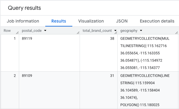
The output is a table of postal codes, their corresponding brand counts, and the postal code geometry.
We can visualize this data as a heatmap. The darker red areas indicate a higher concentration of our target brands, pointing us toward the most commercially dense zones within Las Vegas.
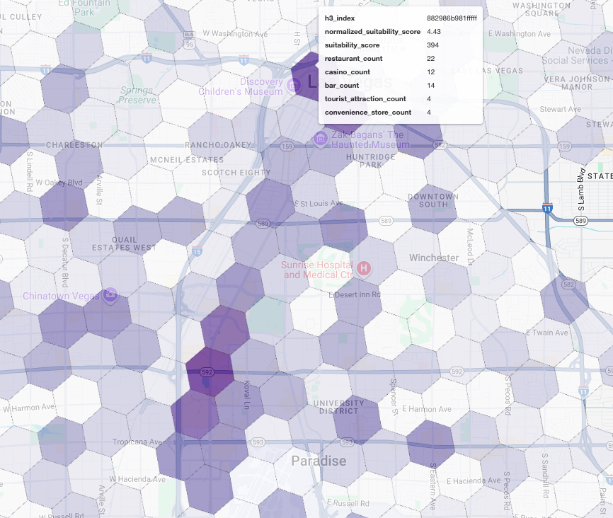
Hyper-Local Analysis: Score Individual Grid Areas
Having identified the general area of Las Vegas, it's time for a granular analysis. This is where we layer in our specific business knowledge. We know a great coffee shop thrives near other businesses that are busy during our peak hours, such as the late-morning and lunch window.
Our next query gets really specific. It starts by creating a fine-grained hexagonal grid over the Las Vegas metropolitan area using the standard H3 geospatial index (at resolution 8) to analyze the area at a micro-level. The query first identifies all complementary businesses that are open during our peak window (Monday, 10 AM to 2 PM).
We then apply a weighted score to each place type. A nearby restaurant is more
valuable to us than a convenience store, so it gets a higher multiplier. This
gives us a custom suitability_score for each small area.
This excerpt highlights the weighted scoring logic, which references a
pre-calculated flag (is_open_monday_window) for the opening hours check:
. . .
(
  COUNTIF('restaurant' IN UNNEST(types) AND is_open_monday_window) * 8 +
  COUNTIF('convenience_store' IN UNNEST(types) AND is_open_monday_window) * 3 +
  COUNTIF('bar' IN UNNEST(types) AND is_open_monday_window) * 7 +
  COUNTIF('tourist_attraction' IN UNNEST(types) AND is_open_monday_window) * 6 +
  COUNTIF('casino' IN UNNEST(types) AND is_open_monday_window) * 7
) AS suitability_score
. . .
Expand for full query
    -- This query calculates a custom 'suitability score' for different areas in the Las Vegas
-- metropolitan area to identify prime commercial zones. It uses a weighted model based
-- on the density of specific business types that are open during a target time window.

-- Step 1: Pre-filter the dataset to only include relevant places.
-- This CTE finds all places in our target localities (Las Vegas, Spring Valley, etc.) and
-- adds a boolean flag 'is_open_monday_window' for those open during the target time.
WITH PlacesInTargetAreaWithOpenFlag AS (
  SELECT
    point,
    types,
    EXISTS(
      SELECT 1
      FROM UNNEST(regular_opening_hours.monday) AS monday_hours
      WHERE
        monday_hours.start_time <= TIME '10:00:00'
        AND monday_hours.end_time >= TIME '14:00:00'
    ) AS is_open_monday_window
  FROM
    `places_insights___us.places`
  WHERE
    EXISTS (
        SELECT 1 FROM UNNEST(locality_names) AS locality
        WHERE locality IN ('Las Vegas', 'Spring Valley', 'Paradise', 'North Las Vegas', 'Winchester')
    )
    AND administrative_area_level_1_name = 'Nevada'
),
-- Step 2: Aggregate the filtered places into H3 cells and calculate the suitability score.
-- Each place's location is converted to an H3 index (at resolution 8). The query then
-- calculates a weighted 'suitability_score' and individual counts for each business type
-- within that cell.
TileScores AS (
  SELECT WITH AGGREGATION_THRESHOLD
    -- Convert each place's geographic point into an H3 cell index.
    `carto-os.carto.H3_FROMGEOGPOINT`(point, 8) AS h3_index,

    -- Calculate the weighted score based on the count of places of each type
    -- that are open during the target window.
    (
      COUNTIF('restaurant' IN UNNEST(types) AND is_open_monday_window) * 8 +
      COUNTIF('convenience_store' IN UNNEST(types) AND is_open_monday_window) * 3 +
      COUNTIF('bar' IN UNNEST(types) AND is_open_monday_window) * 7 +
      COUNTIF('tourist_attraction' IN UNNEST(types) AND is_open_monday_window) * 6 +
      COUNTIF('casino' IN UNNEST(types) AND is_open_monday_window) * 7
    ) AS suitability_score,

    -- Also return the individual counts for each category for detailed analysis.
    COUNTIF('restaurant' IN UNNEST(types) AND is_open_monday_window) AS restaurant_count,
    COUNTIF('convenience_store' IN UNNEST(types) AND is_open_monday_window) AS convenience_store_count,
    COUNTIF('bar' IN UNNEST(types) AND is_open_monday_window) AS bar_count,
    COUNTIF('tourist_attraction' IN UNNEST(types) AND is_open_monday_window) AS tourist_attraction_count,
    COUNTIF('casino' IN UNNEST(types) AND is_open_monday_window) AS casino_count
  FROM
    -- CHANGED: This now references the CTE with the expanded area.
    PlacesInTargetAreaWithOpenFlag
  -- Group by the H3 index to ensure all calculations are per-cell.
  GROUP BY
    h3_index
),
-- Step 3: Find the maximum suitability score across all cells.
-- This value is used in the next step to normalize the scores to a consistent scale (e.g., 0-10).
MaxScore AS (
  SELECT MAX(suitability_score) AS max_score FROM TileScores
)
-- Step 4: Assemble the final results.
-- This joins the scored tiles with the max score, calculates the normalized score,
-- generates the H3 cell's polygon geometry for mapping, and orders the results.
SELECT
  ts.h3_index,
  -- Generate the hexagonal polygon for the H3 cell for visualization.
  `carto-os.carto.H3_BOUNDARY`(ts.h3_index) AS h3_geography,
  ts.restaurant_count,
  ts.convenience_store_count,
  ts.bar_count,
  ts.tourist_attraction_count,
  ts.casino_count,
  ts.suitability_score,
  -- Normalize the score to a 0-10 scale for easier interpretation.
  ROUND(
    CASE
      WHEN ms.max_score = 0 THEN 0
      ELSE (ts.suitability_score / ms.max_score) * 10
    END,
    2
  ) AS normalized_suitability_score
FROM
  -- A cross join is efficient here as MaxScore contains only one row.
  TileScores ts, MaxScore ms
-- Display the highest-scoring locations first.
ORDER BY
  normalized_suitability_score DESC;
Visualizing these scores on a map reveals clear winning locations. The darkest purple tiles, primarily near the Las Vegas Strip and Downtown, are the areas with the highest potential for our new coffee shop.
Competitor Analysis: Identify Existing Coffee Shops
Our suitability model has successfully identified the most promising zones, but a high score alone doesn't guarantee success. We must now overlay this with competitor data. The ideal location is a high-potential area with a low density of existing coffee shops, as we are looking for a clear market gap.
To achieve this, we use the
PLACES_COUNT_PER_H3
function. This function is designed to efficiently return place counts within a
specified geography, by H3 cell.
First, we dynamically define the geography for the entire Las Vegas metro area.
Instead of relying on a single locality, we query the public Overture Maps
dataset to get the boundaries for Las Vegas and its key surrounding localities,
merging them into a single polygon with ST_UNION_AGG. We then pass this area
into the function, asking it to count all operational coffee shops.
This query defines the metro area and calls the function to get coffee shop counts in H3 cells:
-- Define a variable to hold the combined geography for the Las Vegas metro area.
DECLARE las_vegas_metro_area GEOGRAPHY;

-- Set the variable by fetching the shapes for the five localities from Overture Maps
-- and merging them into a single polygon using ST_UNION_AGG.
SET las_vegas_metro_area = (
  SELECT
    ST_UNION_AGG(geometry)
  FROM
    `bigquery-public-data.overture_maps.division_area`
  WHERE
    country = 'US'
    AND region = 'US-NV'
    AND names.primary IN ('Las Vegas', 'Spring Valley', 'Paradise', 'North Las Vegas', 'Winchester')
);

-- Call the PLACES_COUNT_PER_H3 function with our defined area and parameters.
SELECT
  *
FROM
  `places_insights___us.PLACES_COUNT_PER_H3`(
    JSON_OBJECT(
      -- Use the metro area geography we just created.
      'geography', las_vegas_metro_area,
      -- Specify 'coffee_shop' as the place type to count.
      'types', ["coffee_shop"],
      -- Best practice: Only count places that are currently operational.
      'business_status', ['OPERATIONAL'],
      -- Set the H3 grid resolution to 8.
      'h3_resolution', 8
    )
  );
The function returns a table that includes the H3 cell index, its geometry, the total count of coffee shops, and a sample of their Place IDs:
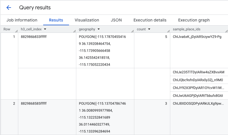
While the aggregate count is useful, seeing the actual competitors is essential.
This is where we transition from the Places Insights dataset to the Places
API. By extracting the
sample_place_ids from the cells with the highest normalized suitability score,
we can call Place Details
API to retrieve rich
details for each competitor, such as their name, address, rating, and location.
This requires comparing the results of the previous query, where the suitability
score was generated, and the PLACES_COUNT_PER_H3 query. The H3 Cell Index can
be used to get the coffee shop counts and IDs from the cells with the highest
normalized suitability score.
This Python code demonstrates how this comparison could be performed.
    # Isolate the Top 5 Most Suitable H3 Cells
    top_suitability_cells = gdf_suitability.head(5)

    # Extract the 'h3_index' values from these top 5 cells into a list.
    top_h3_indexes = top_suitability_cells['h3_index'].tolist()
    print(f"The top 5 H3 indexes are: {top_h3_indexes}")

    # Now, we find the rows in our DataFrame where the
    # 'h3_cell_index' matches one of the indexes from our top 5 list.

    coffee_counts_in_top_zones = gdf_coffee_shops[
        gdf_coffee_shops['h3_cell_index'].isin(top_h3_indexes)
    ]
Now we have the list of Place IDs for coffee shops that already exist within the H3 cells with the highest suitability score, further details about each place can be requested.
This can be done by either sending a request to the Place Details
API directly for each
Place ID, or using a Client
Library to perform the
call. Remember to set the
FieldMask
parameter to only request the data you need.
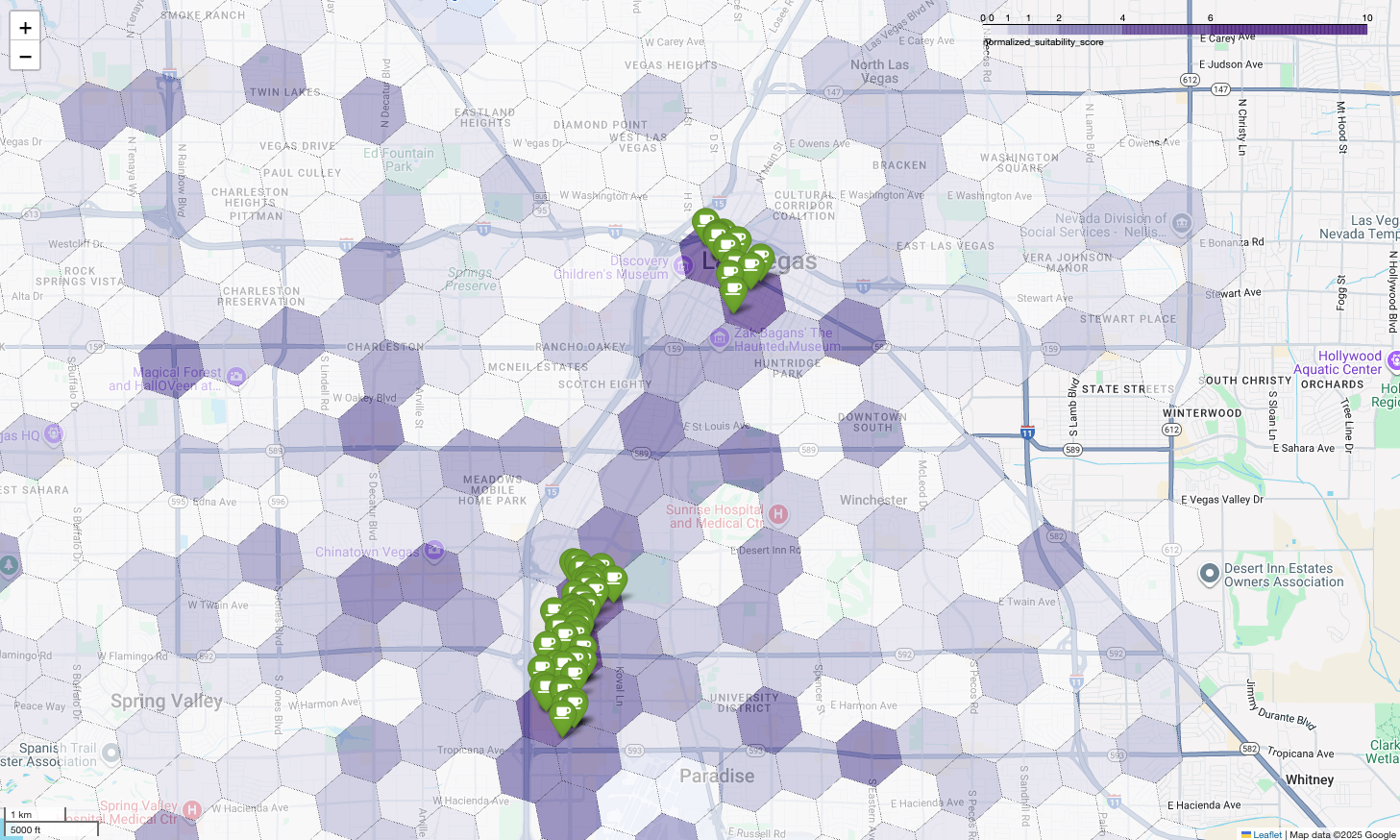
Finally, we combine everything into a single, powerful visualization. We plot our purple suitability choropleth map as the base layer and then add pins for each individual coffee shop retrieved from the Places API. This final map provides an at-a-glance view that synthesizes our entire analysis: the dark purple areas show the potential, and the green pins show the reality of the current market.
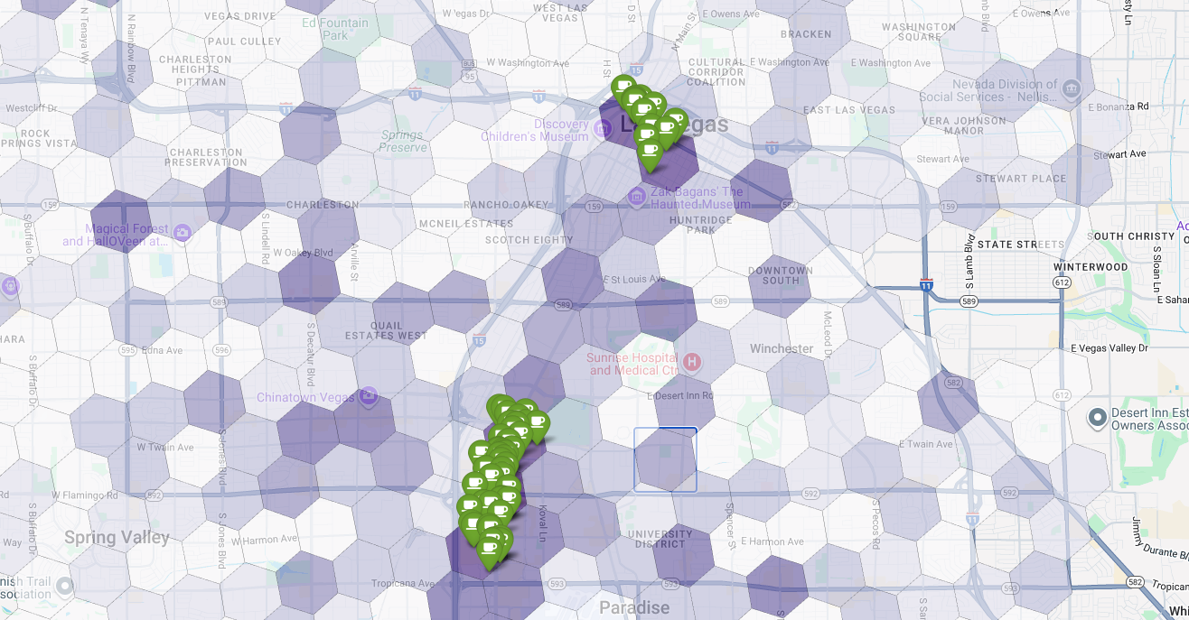
By looking for dark purple cells with few or no pins, we can confidently pinpoint the exact areas that represent the best opportunity for our new location.
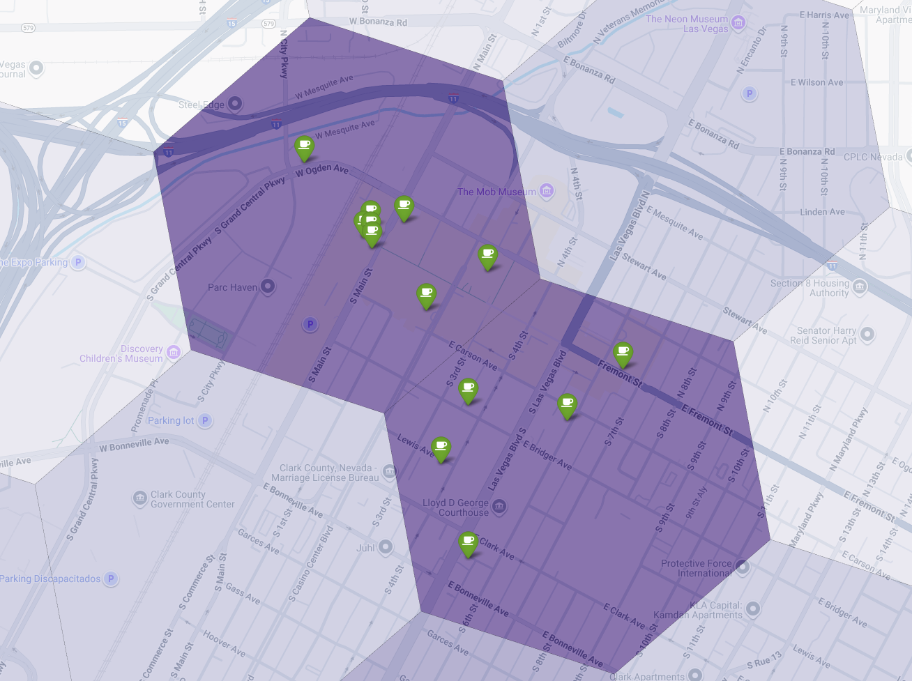
The above two cells have a high suitability score, but some clear gaps that could be potential locations for our new coffee shop.
Conclusion
In this document, we moved from a state-wide question of where to expand? to a data-backed, local answer. By layering different datasets and applying custom business logic, you can systematically reduce the risk associated with a major business decision. This workflow, combining the scale of BigQuery, the richness of Places Insights, and the real-time detail of the Places API, provides a powerful template for any organization looking to use location intelligence for strategic growth.
Next steps
- Adapt this workflow with your own business logic, target geographies, and proprietary datasets.
- Explore other data fields in the Places Insights dataset, such as review counts, price levels, and user ratings, to further enrich your model.
- Automate this process to create an internal site selection dashboard that can be used to evaluate new markets dynamically.
Dive deeper into the documentation:
Contributors
Henrik Valve | DevX Engineer