Validate Places Insights data using sample Place IDs

In this document, you will learn how to use sample Place IDs data from Places Insights, using Place Count Functions, alongside targeted Place Details lookups to build confidence in your results.

The Architectural Pattern

This architectural pattern gives you a repeatable workflow to bridge the gap between high-level statistical analysis and ground-truth verification. By combining the scale of BigQuery with the precision of the Places API, you can confidently validate your analytical findings. This is particularly useful for site selection, competitor analysis, and market research where trust in the data is paramount.

The core of this pattern involves four key steps:

1. Perform Large-Scale Analysis: Use a Place Count Function from Places Insights in BigQuery to analyze place data over a large geography, such as an entire city or region.
2. Isolate and Extract Samples: Identify areas of interest (e.g., "hotspots" with high density) from the aggregated results and extract the sample_place_ids provided by the function.
3. Retrieve Ground-Truth Details: Use the extracted Place IDs to make targeted calls to the Place Details API to fetch rich, real-world details for each place.
4. Create a Combined Visualization: Layer the detailed place data on top of the initial high-level statistical map to visually validate that the aggregated counts reflect reality on the ground.

Solution Workflow

This workflow lets you to bridge the gap between macro-level trends and micro-level facts. You start with a broad, statistical view and strategically drill down to verify the data with specific, real-world examples.

Analyze Place Density at Scale with Places Insights

Your first step is to understand the landscape at a high level. Instead of fetching thousands of individual points of interest (POIs), you can run a single query to get a statistical summary.

The Places Insights PLACES_COUNT_PER_H3 function is ideal for this. It aggregates POI counts into a hexagonal grid system (H3), allowing you to quickly identify areas of high or low density based on your specific criteria (e.g., restaurants with a high rating that are operational).

An example query is as follows. Note that you will be required to provide your search area geography. An open dataset, such as the Overture Maps Data BigQuery public dataset can be used to retrieve geographical boundary data.

For frequently used open dataset boundaries, we recommend materializing them into a table in your own project. This significantly reduces BigQuery costs and improves query performance.

-- This query counts all highly-rated, operational restaurants
-- across a large geography, grouping them into H3 cells.
SELECT *
FROM
  `places_insights___gb.PLACES_COUNT_PER_H3`(
    JSON_OBJECT(
      'geography', your_defined_geography,
      'h3_resolution', 8,
      'types', ['restaurant'],
      'business_status', ['OPERATIONAL'],
      'min_rating', 3.5
    )
  );

The output of this query gives you a table of H3 cells and the count of places within each, forming the basis for a density heatmap.

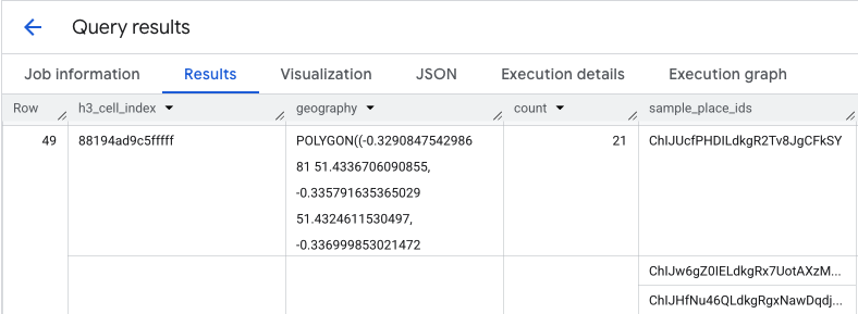
Isolate Hotspots and Extract Sample Place IDs

The result from the PLACES_COUNT_PER_H3 function also returns an array of sample_place_ids, up to 250 Place IDs per element of the response. These IDs are the link from the aggregated statistic to the individual places that contribute to it.

Your system could first identify the most relevant cells from the initial query. For example, you might select the top 20 cells with the highest counts. Then, from these hotspots, you consolidate the sample_place_ids into a single list. This list represents a curated sample of the most interesting POIs from the most relevant areas, preparing you for targeted verification.

If you are processing your BigQuery results in Python using a pandas DataFrame, the logic to extract these IDs is straightforward:

# Assume 'results_df' is a pandas DataFrame from your BigQuery query.

# 1. Identify the 20 busiest H3 cells by sorting and taking the top results.
top_hotspots_df = results_df.sort_values(by='count', ascending=False).head(20)

# 2. Extract and flatten the lists of sample_place_ids from these hotspots.
# The .explode() function creates a new row for each ID in the lists.
all_sample_ids = top_hotspots_df['sample_place_ids'].explode()

# 3. Create a final list of unique Place IDs to verify.
place_ids_to_verify = all_sample_ids.unique().tolist()

print(f"Consolidated {len(place_ids_to_verify)} unique Place IDs for spot-checking.")

Similar logic can be applied if using other programming languages.

Retrieve Ground-Truth Details with the Places API

Tip: Geocoding API also supports using Place IDs to retrieve place information.

With your consolidated list of Place IDs, you now transition from large-scale analytics to specific data retrieval. You will use these IDs to query the Place Details API for detailed information on each sample location.

This is a critical validation step. While Places Insights told you how many restaurants were in an area, the Places API tells you which restaurants they are, providing their name, exact address, latitude/longitude, user rating, and even a direct link to their location on Google Maps. This enriches your sample data, turning abstract IDs into concrete, verifiable places.

For the full list of data available from Place Details API, and the cost associated with retrieval, review the API documentation. The FieldMask is set on the request, to control the data returned from the API.

A request to the Places API for a specific ID using the Python client library would look like this:

# A request to fetch details for a single Place ID.
request = {"name": f"places/{place_id}"}

# Define the fields you want returned in the response as a comma-separated string.
fields_to_request = "displayName,formattedAddress,location,googleMapsUri"

# The response contains ground truth data.
response = places_client.get_place(
    request=request,
    metadata=[("x-goog-fieldmask", fields_to_request)]
)

See Places API (New) client library examples for more details.

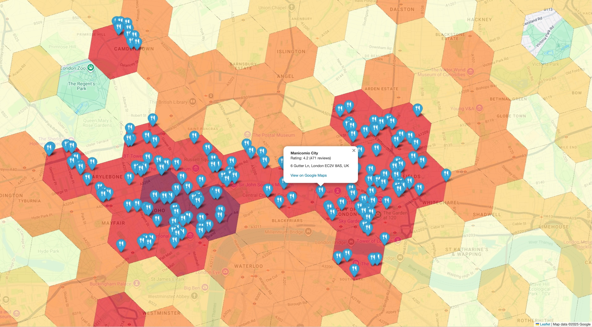
Create a Combined Visualization for Validation

Tip: Places UI Kit can also be used to visualize results using Place IDs.

The final step is to bring both datasets together in a single view. This provides an immediate and intuitive way to spot-check your initial analysis. Your visualization should have two layers:

1. Base Layer: A choropleth or heatmap generated from the initial PLACES_COUNT_PER_H3 results, showing the overall density of places across your geography.
2. Top Layer: A set of individual markers for each sample POI, plotted using the precise coordinates retrieved from the Places API in the previous step.

The logic for building this combined view is expressed in this pseudo-code example:

# Assume 'h3_density_data' is your aggregated data from Step 1.
# Assume 'detailed_places_data' is your list of place objects from Step 3.

# Create the base choropleth map from the H3 density data.
# The 'count' column determines the color of each hexagon.
combined_map = create_choropleth_map(
    data=h3_density_data,
    color_by_column='count'
)

# Iterate through the detailed place data to add individual markers.
for place in detailed_places_data:
    # Construct the popup information with key details and a link.
    popup_html = f"""
    <b>{place.name}</b><br>
    Address: {place.address}<br>
    <a href="{place.google_maps_uri}" target="_blank">View on Maps</a>
    """

    # Add a marker for the current place to the base map.
    combined_map.add_marker(
        location=[place.latitude, place.longitude],
        popup=popup_html,
        tooltip=place.name
    )

# Display the final map with both layers.
display(combined_map)

By overlaying the specific, ground-truth markers on the high-level density map, you can instantly confirm that the areas identified as hotspots do, in fact, contain a high concentration of the places you're analyzing. This visual confirmation builds significant trust in your data-driven conclusions.

Conclusion

This architectural pattern provides a robust and efficient method for validating large-scale geospatial insights. By leveraging Places Insights for broad, scalable analysis and the Place Details API for targeted, ground-truth verification, you create a powerful feedback loop. This ensures your strategic decisions, whether in retail site selection or logistics planning, are based on data that is not only statistically significant but also verifiably accurate.

Next steps

• Explore other Place Count Functions to see how they can answer different analytical questions.
• Review the Places API documentation to discover other fields you can request to further enrich your analysis.

Contributors

Henrik Valve | DevX Engineer