Page Summary
-
Earth Engine provides various spectral transformation methods such as
normalizedDifference(),unmix(),rgbToHsv(), andhsvToRgb(). -
Pan sharpening improves image resolution by combining a multiband image with a higher-resolution panchromatic image, often using
rgbToHsv()andhsvToRgb(). -
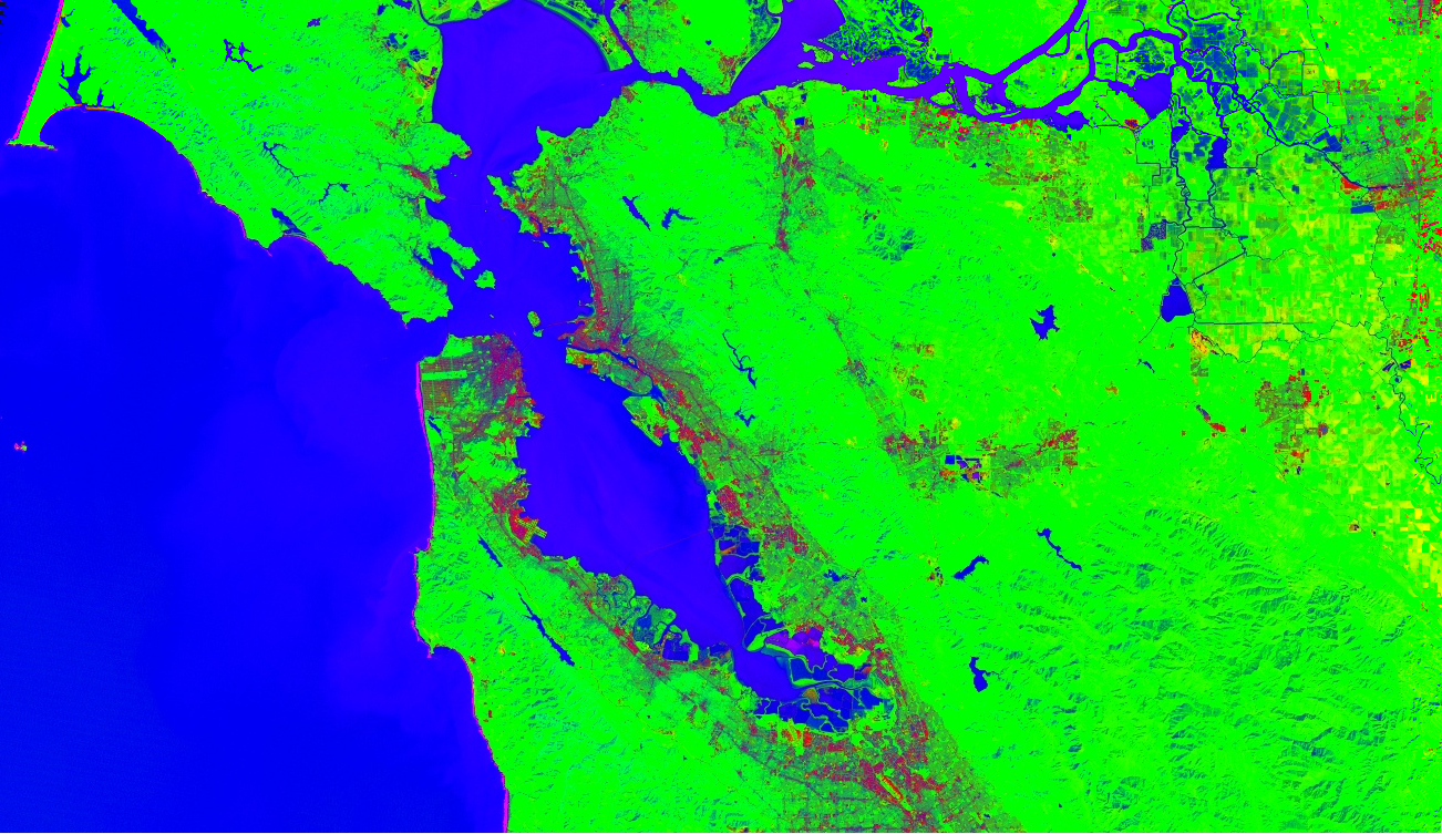
Spectral unmixing, implemented as
image.unmix(), separates a pixel's spectrum into fractional components based on defined endmembers.
 View source on GitHub
There are several spectral transformation methods in Earth Engine. These include instance
methods on images such as normalizedDifference(), unmix(),
rgbToHsv() and hsvToRgb().
Pan sharpening
Pan sharpening improves the resolution of a multiband image through
enhancement provided by a corresponding panchromatic image with finer resolution.
The rgbToHsv() and hsvToRgb() methods are useful for pan
sharpening.
Code Editor (JavaScript)
// Load a Landsat 8 top-of-atmosphere reflectance image.
var image = ee.Image('LANDSAT/LC08/C02/T1_TOA/LC08_044034_20140318');
Map.addLayer(
    image,
    {bands: ['B4', 'B3', 'B2'], min: 0, max: 0.25, gamma: [1.1, 1.1, 1]},
    'rgb');

// Convert the RGB bands to the HSV color space.
var hsv = image.select(['B4', 'B3', 'B2']).rgbToHsv();

// Swap in the panchromatic band and convert back to RGB.
var sharpened = ee.Image.cat([
  hsv.select('hue'), hsv.select('saturation'), image.select('B8')
]).hsvToRgb();

// Display the pan-sharpened result.
Map.setCenter(-122.44829, 37.76664, 13);
Map.addLayer(sharpened,
             {min: 0, max: 0.25, gamma: [1.3, 1.3, 1.3]},
             'pan-sharpened');
import ee
import geemap.core as geemap
Colab (Python)
# Load a Landsat 8 top-of-atmosphere reflectance image.
image = ee.Image('LANDSAT/LC08/C02/T1_TOA/LC08_044034_20140318')

# Convert the RGB bands to the HSV color space.
hsv = image.select(['B4', 'B3', 'B2']).rgbToHsv()

# Swap in the panchromatic band and convert back to RGB.
sharpened = ee.Image.cat(
    [hsv.select('hue'), hsv.select('saturation'), image.select('B8')]
).hsvToRgb()

# Define a map centered on San Francisco, California.
map_sharpened = geemap.Map(center=[37.76664, -122.44829], zoom=13)

# Add the image layers to the map and display it.
map_sharpened.add_layer(
    image,
    {
        'bands': ['B4', 'B3', 'B2'],
        'min': 0,
        'max': 0.25,
        'gamma': [1.1, 1.1, 1],
    },
    'rgb',
)
map_sharpened.add_layer(
    sharpened,
    {'min': 0, 'max': 0.25, 'gamma': [1.3, 1.3, 1.3]},
    'pan-sharpened',
)
display(map_sharpened)
Spectral unmixing
Spectral unmixing is implemented in Earth Engine as the image.unmix() method.
(For more flexible methods, see the Array Transformations
page). The following is an example of unmixing Landsat 5 with predetermined urban,
vegetation and water endmembers:
Code Editor (JavaScript)
// Load a Landsat 5 image and select the bands we want to unmix.
var bands = ['B1', 'B2', 'B3', 'B4', 'B5', 'B6', 'B7'];
var image = ee.Image('LANDSAT/LT05/C02/T1/LT05_044034_20080214')
  .select(bands);
Map.setCenter(-122.1899, 37.5010, 10); // San Francisco Bay
Map.addLayer(image, {bands: ['B4', 'B3', 'B2'], min: 0, max: 128}, 'image');

// Define spectral endmembers.
var urban = [88, 42, 48, 38, 86, 115, 59];
var veg = [50, 21, 20, 35, 50, 110, 23];
var water = [51, 20, 14, 9, 7, 116, 4];

// Unmix the image.
var fractions = image.unmix([urban, veg, water]);
Map.addLayer(fractions, {}, 'unmixed');
import ee
import geemap.core as geemap
Colab (Python)
# Load a Landsat 5 image and select the bands we want to unmix.
bands = ['B1', 'B2', 'B3', 'B4', 'B5', 'B6', 'B7']
image = ee.Image('LANDSAT/LT05/C02/T1/LT05_044034_20080214').select(bands)

# Define spectral endmembers.
urban = [88, 42, 48, 38, 86, 115, 59]
veg = [50, 21, 20, 35, 50, 110, 23]
water = [51, 20, 14, 9, 7, 116, 4]

# Unmix the image.
fractions = image.unmix([urban, veg, water])

# Define a map centered on San Francisco Bay.
map_fractions = geemap.Map(center=[37.5010, -122.1899], zoom=10)

# Add the image layers to the map and display it.
map_fractions.add_layer(
    image, {'bands': ['B4', 'B3', 'B2'], 'min': 0, 'max': 128}, 'image'
)
map_fractions.add_layer(fractions, None, 'unmixed')
display(map_fractions)