Page Summary
-
Image linear convolutions are performed using
image.convolve()with anee.Kernelargument defined by a shape and weights. -
Kernels are applied to each image band individually and their size and coefficients are determined by parameters like
radius,units, andnormalize. -
Different kernels, such as low-pass for smoothing or Laplacian for edge detection, can be used to achieve desired image processing effects.
-
Anisotropic edge detection kernels can be rotated, and custom kernels with arbitrary weights and shapes can be created using
ee.Kernel.fixed().
To perform linear convolutions on images, use image.convolve(). The only
argument to convolve is an ee.Kernel which is specified by a shape and the
weights in the kernel. Each pixel of the image output by convolve()
is the linear combination of the kernel values and the input image pixels covered by the
kernel. The kernels are applied to each band individually. For example, you might want
to use a low-pass (smoothing) kernel to remove high-frequency information. The following
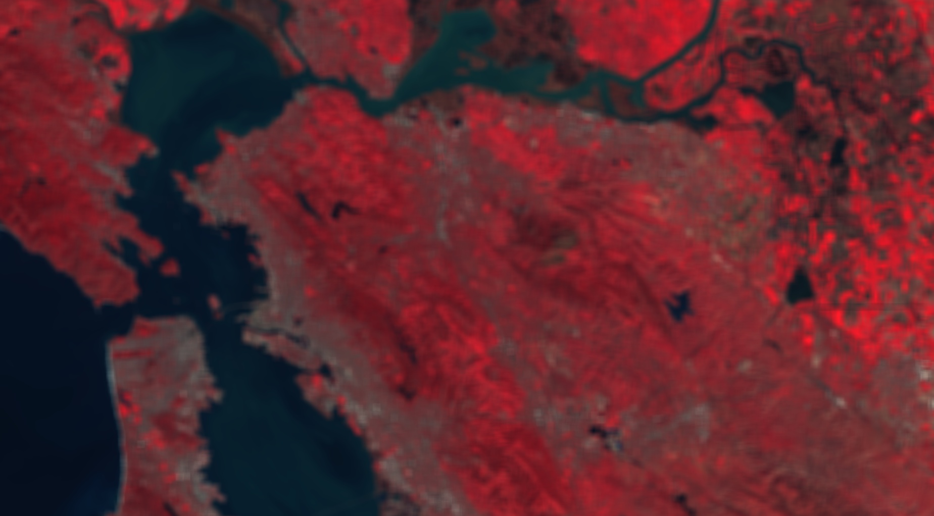
illustrates a 15x15 low-pass kernel applied to a Landsat 8 image:
Code Editor (JavaScript)
// Load and display an image.
var image = ee.Image('LANDSAT/LC08/C02/T1_TOA/LC08_044034_20140318');
Map.setCenter(-121.9785, 37.8694, 11);
Map.addLayer(image, {bands: ['B5', 'B4', 'B3'], max: 0.5}, 'input image');

// Define a boxcar or low-pass kernel.
var boxcar = ee.Kernel.square({
  radius: 7, units: 'pixels', normalize: true
});

// Smooth the image by convolving with the boxcar kernel.
var smooth = image.convolve(boxcar);
Map.addLayer(smooth, {bands: ['B5', 'B4', 'B3'], max: 0.5}, 'smoothed');
The output of convolution with the low-pass filter should look something like Figure
1. Observe that the arguments to the kernel determine its size and coefficients.
Specifically, with the units parameter set to pixels, the radius
parameter specifies the number of pixels from the center that the kernel will cover. If
normalize is set to true, the kernel coefficients will sum to one. If
the magnitude parameter is set, the kernel coefficients will be multiplied by
the magnitude (if normalize is also true, the coefficients will sum to
magnitude). If there is a negative value in any of the kernel coefficients,
setting normalize to true will make the coefficients sum to zero.
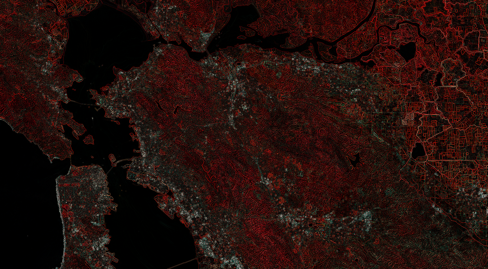
Use other kernels to achieve the desired image processing effect. This example uses a Laplacian kernel for isotropic edge detection:
Code Editor (JavaScript)
// Define a Laplacian, or edge-detection kernel.
var laplacian = ee.Kernel.laplacian8({ normalize: false });

// Apply the edge-detection kernel.
var edgy = image.convolve(laplacian);
Map.addLayer(edgy,
             {bands: ['B5', 'B4', 'B3'], max: 0.5, format: 'png'},
             'edges');
Note the format specifier in the visualization parameters. Earth Engine sends display tiles to the Code Editor in JPEG format for efficiency, however edge tiles are sent in PNG format to handle transparency of pixels outside the image boundary. When a visual discontinuity results, setting the format to PNG results in a consistent display. The result of convolving with the Laplacian edge detection kernel should look something like Figure 2.
There are also anisotropic edge detection kernels (e.g. Sobel, Prewitt, Roberts), the
direction of which can be changed with kernel.rotate(). Other low pass
kernels include a Gaussian kernel and kernels of various shape with uniform weights. To
create kernels with arbitrarily defined weights and shape, use
ee.Kernel.fixed(). For example, this code creates a 9x9 kernel of 1’s
with a zero in the middle:
Code Editor (JavaScript)
// Create a list of weights for a 9x9 kernel.
var row = [1, 1, 1, 1, 1, 1, 1, 1, 1];
// The center of the kernel is zero.
var centerRow = [1, 1, 1, 1, 0, 1, 1, 1, 1];
// Assemble a list of lists: the 9x9 kernel weights as a 2-D matrix.
var rows = [row, row, row, row, centerRow, row, row, row, row];
// Create the kernel from the weights.
var kernel = ee.Kernel.fixed(9, 9, rows, -4, -4, false);
print(kernel);