
The PLACES_COUNT_V2 function returns a BigQuery table containing place counts
and sample Place IDs for multiple input geographies based on specified filters.
This function is designed for efficient batch processing by accepting an input
table
parameter
of geographies, allowing you to analyze many areas of interest in a single query
by providing the geographies through an input table.
Syntax
SELECT * FROM `PROJECT_NAME.LINKED_DATASET_NAME.PLACES_COUNT_V2`(
  TABLE input_geographies,
  filters
)
Parameters
PROJECT_NAME: The name of your Google Cloud project.LINKED_DATASET_NAME: The name of the BigQuery dataset containing the Places Insights functions (e.g.,places_insights___us).input_geographies: A BigQuery table containing the geographies to analyze. This table must include the following columns:filters(JSON): A JSON object containing key-value pairs for filtering the places. See Filter Parameters.
Output Table Schema
The PLACES_COUNT_V2 function returns a table with the following columns:
| Column Name | Data Type | Description |
|---|---|---|
geo_id |
STRING | The unique identifier for the input geography, from the input_geographies table. |
input_geography |
GEOGRAPHY | The original GEOGRAPHY object from the input_geographies table. |
place_count |
INTEGER | The total number of places matching the filters. |
sample_place_ids |
ARRAY<STRING> | An array of up to 250 Place IDs that match the criteria. |
How it works
The function processes each row in the input_geographies table. For each geo
object, it counts the number of places that fall within the geography (or within
the geography_radius if the geo is a point and the radius is specified in
the filters). The count includes only those places that match all the
conditions defined in the filters JSON object.
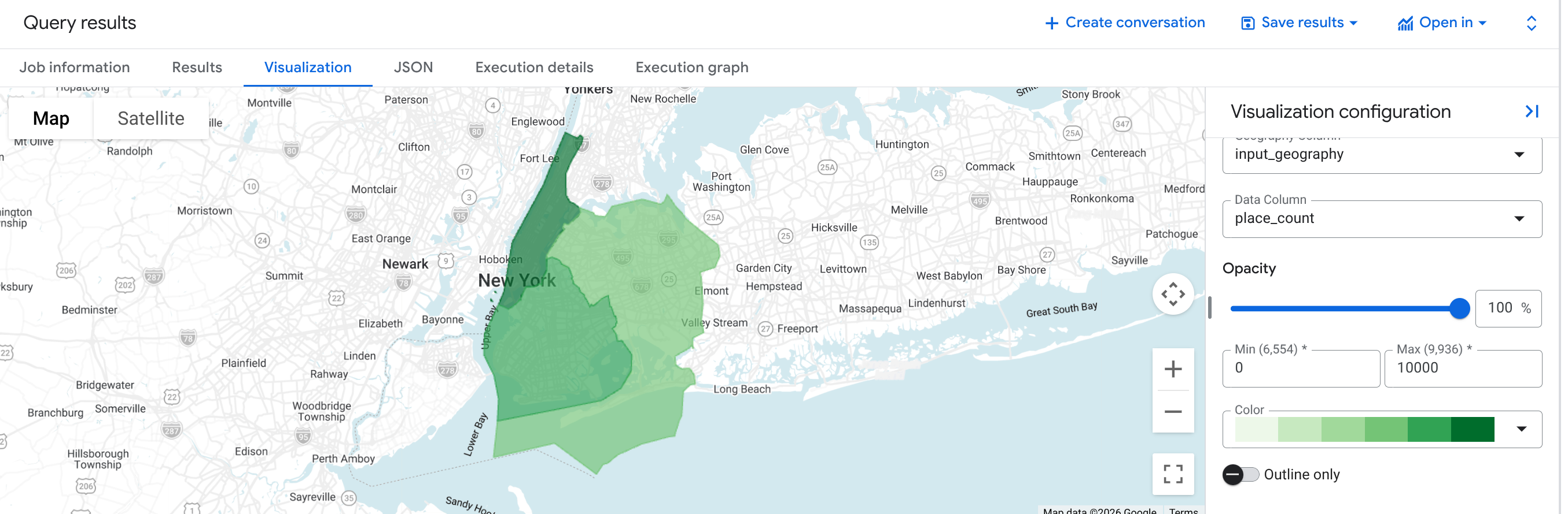
Example: Calculate the number of restaurants in three counties of New York City
This example generates a table of the number of operational restaurants in three counties of New York City.
This example uses the United States Census Bureau
Data
BigQuery public dataset to get
the boundaries for three counties in New York City: "Queens", "Kings", and "New
York". The boundaries of each county are contained in the county_geom column.
We first create a temporary table new_york_counties to hold the geo_id and
the simplified GEOGRAPHY for each county.
SELECT *
FROM `PROJECT_NAME.places_insights___us.PLACES_COUNT_V2`(
  (
    SELECT
      county_name AS geo_id,
      ST_SIMPLIFY(county_geom, 100) AS geo
    FROM
      `bigquery-public-data.geo_us_boundaries.counties`
    WHERE
      state_fips_code = "36"  -- New York State
      AND county_name IN ("Queens", "Kings", "New York")
  ),
  JSON_OBJECT(
      'types', ["restaurant"],
      'business_status', ['OPERATIONAL']
  )
);
The response table will have three rows, one for each county, showing the
geo_id, input_geography, place_count, and sample_place_ids of
operational restaurants.
Benefits of using PLACES_COUNT_V2
PLACES_COUNT_V2 offers significant advantages over both PLACES_COUNT and
PLACES_COUNT_PER_GEO:
- Batch Processing: Efficiently analyze thousands of custom geographies in a single query by supplying multiple geography inputs in a table.
- Performance: Utilizes BigQuery's optimized geospatial joins offering significant speed advantages for large datasets.
- Scalability: Designed to handle a large number of input geographies without the limitations of single JSON parameter size.
- Zero Counts Included:
PLACES_COUNT_V2returns a row for everygeo_idprovided in the input table. If no places match the criteria for a given geography, theplace_countwill be 0. This ensures you have a result for each input area, so you can see where places are absent.