Page Summary
-
Gradient boosted trees, unlike random forests, are susceptible to overfitting and may require regularization and early stopping techniques using a validation dataset.
-
Key regularization parameters for gradient boosted trees include maximum tree depth, shrinkage rate, attribute test ratio at each node, and L1/L2 coefficients on the loss.
-
Gradient boosted trees offer advantages such as native support for various feature types, generally good default hyperparameters, and efficient model size and prediction speed.
-
Training gradient boosted trees involves sequential tree construction, potentially slowing down the process, and they lack the ability to learn and reuse internal representations, potentially impacting performance on certain datasets.
Unlike random forests, gradient boosted trees can overfit. Therefore, as for neural networks, you can apply regularization and early stopping using a validation dataset.
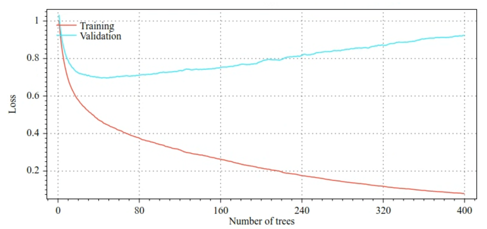
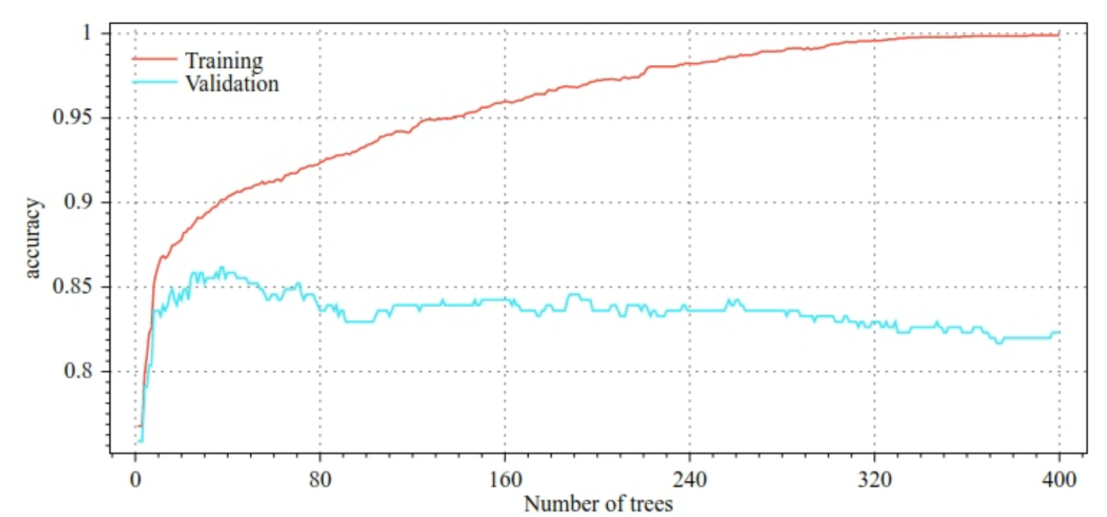
For example, the following figures show loss and accuracy curves for training and validation sets when training a GBT model. Notice how divergent the curves are, which suggests a high degree of overfitting.

Figure 29. Loss vs. number of decision trees.

Figure 30. Accuracy vs. number of decision trees.
Common regularization parameters for gradient boosted trees include:
- The maximum depth of the tree.
- The shrinkage rate.
- The ratio of attributes tested at each node.
- L1 and L2 coefficient on the loss.
Note that decision trees generally grow much shallower than random forest models. By default, gradient boosted trees trees in TF-DF are grown to depth 6. Because the trees are shallow, the minimum number of examples per leaf has little impact and is generally not tuned.
The need for a validation dataset is an issue when the number of training examples is small. Therefore, it is common to train gradient boosted trees inside a cross-validation loop, or to disable early stopping when the model is known not to overfit.
Usage example
In the previous chapter, we trained a random forest on a small dataset. In this example, we will simply replace the random forest model with a gradient boosted trees model:
model = tfdf.keras.GradientBoostedTreesModel()

# Part of the training dataset will be used as validation (and removed
# from training).
model.fit(tf_train_dataset)

# The user provides the validation dataset.
model.fit(tf_train_dataset, validation_data=tf_valid_dataset)

# Disable early stopping and the validation dataset. All the examples are
# used for training.
model.fit(
   tf_train_dataset,
   validation_ratio=0.0,
   early_stopping="NONE")
# Note: When "validation_ratio=0", early stopping is automatically disabled,
# so early_stopping="NONE" is redundant here.
Usage and limitations
Gradient boosted trees have some pros and cons.
Pros
- Like decision trees, they natively support numerical and categorical features and often do not need feature pre-processing.
- Gradient boosted trees have default hyperparameters that often give great results. Nevertheless, tuning those hyperparameters can significantly improve the model.
- Gradient boosted tree models are generally small (in number of nodes and in memory) and fast to run (often just one or a few µs / examples).
Cons
- The decision trees must be trained sequentially, which can slow training considerably. However, the training slowdown is somewhat offset by the decision trees being smaller.
- Like random forests, gradient boosted trees can't learn and reuse internal representations. Each decision tree (and each branch of each decision tree) must relearn the dataset pattern. In some datasets, notably datasets with unstructured data (for example, images, text), this causes gradient boosted trees to show poorer results than other methods.