Page Summary
-
Decision trees are trained using heuristics due to the complexity of finding the optimal tree structure.
-
A greedy divide-and-conquer strategy recursively grows the tree by selecting the "best" condition at each node.
-
Splitters are algorithms responsible for finding the best condition, optimizing for metrics like information gain or mean squared error depending on the task.
-
The choice of splitter algorithm depends on factors such as feature type, task, condition type, and regularization criteria.
-
YDF automatically selects splitters based on feature type, hyperparameters, and estimated speed.
Like all supervised machine learning models, decision trees are trained to best explain a set of training examples. The optimal training of a decision tree is an NP-hard problem. Therefore, training is generally done using heuristics—an easy-to-create learning algorithm that gives a non-optimal, but close to optimal, decision tree.
Most algorithms used to train decision trees work with a greedy divide and conquer strategy. The algorithm starts by creating a single node (the root) and recursively and greedily grows the decision tree.
At each node, all the possible conditions are evaluated and scored. The algorithm selects the "best" condition, that is, the condition with the highest score. For now, just know that the score is a metric that correlates with the task, and conditions are selected to maximize that metric.
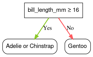
For example, in the Palmer Penguins dataset (used for code examples later in this course), most Adelie and Chinstrap penguins have a bill's length greater than 16mm, while most of the Gentoo penguins have smaller bills. Therefore, the condition bill_length_mm ≥ 16 makes almost perfect predictions for the Gentoo penguins, but can't differentiate between Adelies and Chinstraps. The algorithm will probably pick this condition.

Figure 7. The first step in growing a tree.
The algorithm then repeats recursively and independently on both children nodes. When no satisfying conditions are found, the node becomes a leaf. The leaf prediction is determined as the most representative label value in the examples.
The algorithm is as follows:
def train_decision_tree(training_examples):
  root = create_root() # Create a decision tree with a single empty root.
  grow_tree(root, training_examples) # Grow the root node.
  return root

def grow_tree(node, examples):
  condition = find_best_condition(examples) # Find the best condition.

  if condition is None:
    # No satisfying conditions were found, therefore the grow of the branch stops.
    set_leaf_prediction(node, examples)
    return

  # Create two childrens for the node.
  positive_child, negative_child = split_node(node, condition)

  # List the training examples used by each children.
  negative_examples = [example for example in examples if not condition(example)]
  positive_examples = [example for example in examples if condition(example)]

  # Continue the growth of the children.
  grow_tree(negative_child, negative_examples)
  grow_tree(positive_child, positive_examples)
Let's go through the steps of training a particular decision tree in more detail.
Step 1: Create a root:

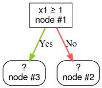
Step 2: Grow node #1. The condition "x1 ≥ 1" was found. Two child nodes are created:

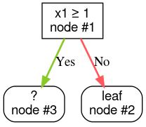
Step 3: Grow node #2. No satisfying conditions were found. So, make the node into a leaf:

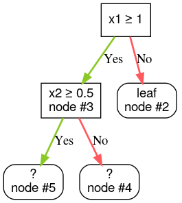
Step 4: Grow node #3. The condition "x2 ≥ 0.5" was found. Two child nodes are created.

Other methods exist to grow decision trees. A popular alternative is to optimize nodes globally instead of using a divide and conquer strategy.
growing_strategy="BEST_FIRST_GLOBAL" parameter.
See
the documentation for more details.
Depending on the number and type of input features, the number of possible conditions for a given node can be huge, generally infinite. For example, given a threshold condition $\mathrm{feature}_i \geq t$, the combination of all the possible threshold values for $t \in \mathbb{R}$ is infinite.
The routine responsible for finding the best condition is called the splitter. Because it needs to test a lot of possible conditions, splitters are the bottleneck when training a decision tree.
The score maximized by the splitter depends on the task. For example:
- Information gain and Gini (both covered later) are commonly used for classification.
- Mean squared error is commonly used for regression.
There are many splitter algorithms, each with varying support for:
- The type of features; for example, numerical, categorical, text
- The task; for example, binary classification, multi-class classification, regression
- The type of condition; for example, threshold condition, in-set condition, oblique condition
- The regularization criteria; for example, exact or approximated splitters for threshold conditions
In addition, there are equivalent splitter variants with different trade-offs regarding memory usage, CPU usage, computation distribution, and so on.