Page Summary
-
Gradient boosting creates a strong predictive model by iteratively combining multiple weak models, typically decision trees.
-
In each iteration, a new weak model is trained to predict the errors of the current strong model, and then added to the strong model to improve its accuracy.
-
Shrinkage, similar to learning rate in neural networks, is used to control the learning speed and prevent overfitting by scaling the contribution of each weak model.
-
Gradient boosted trees are a specific implementation of gradient boosting that utilizes decision trees as the weak learners.
-
TensorFlow Decision Forests provides a practical implementation through
tfdf.keras.GradientBoostedTreeModel, streamlining the model building process.
Like bagging and boosting, gradient boosting is a methodology applied on top of another machine learning algorithm. Informally, gradient boosting involves two types of models:
- a "weak" machine learning model, which is typically a decision tree.
- a "strong" machine learning model, which is composed of multiple weak models.
In gradient boosting, at each step, a new weak model is trained to predict the "error" of the current strong model (which is called the pseudo response). We will detail "error" later. For now, assume "error" is the difference between the prediction and a regressive label. The weak model (that is, the "error") is then added to the strong model with a negative sign to reduce the error of the strong model.
Gradient boosting is iterative. Each iteration invokes the following formula:
\[ F_{i+1} = F_i - f_i \]
where:
- $F_i$ is the strong model at step $i$.
- $f_i$ is the weak model at step $i$.
This operation repeats until a stopping criterion is met, such as a maximum number of iterations or if the (strong) model begins to overfit as measured on a separate validation dataset.
Let's illustrate gradient boosting on a simple regression dataset where:
- The objective is to predict $y$ from $x$.
- The strong model is initialized to be a zero constant: $F_0(x) = 0$.
# Simplified example of regressive gradient boosting.

y = ... # the labels
x = ... # the features

strong_model = []
strong_predictions = np.zeros_like(y) # Initially, the strong model is empty.

for i in range(num_iters):

    # Error of the strong model
    error = strong_predictions - y

    # The weak model is a decision tree (see CART chapter)
    # without pruning and a maximum depth of 3.
    weak_model = tfdf.keras.CartModel(
        task=tfdf.keras.Task.REGRESSION,
        validation_ratio=0.0,
        max_depth=3)
    weak_model.fit(x=x, y=error)

    strong_model.append(weak_model)

    weak_predictions = weak_model.predict(x)[:,0]

    strong_predictions -= weak_predictions
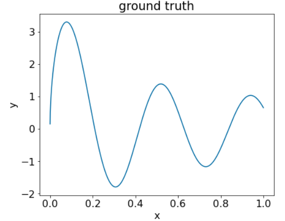
Let's apply this code on the following dataset:

Figure 25. A synthetic regressive dataset with one numerical feature.
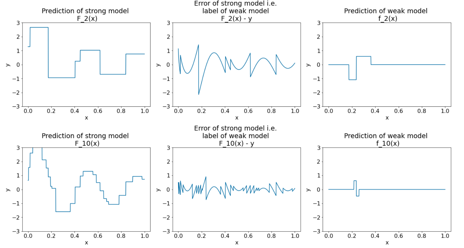
Here are three plots after the first iteration of the gradient boosting algorithm:

Figure 26. Three plots after the first iteration.
Note the following about the plots in Figure 26:
- The first plot shows the predictions of the strong model, which is currently always 0.
- The second plot shows the error, which is the label of the weak model.
- The third plot shows the weak model.
The first weak model is learning a coarse representation of the label and mostly focuses on the left part of the feature space (the part with the most variation, and therefore the most error for the constant wrong model).
Following are the same plots for another iteration of the algorithm:

Figure 27. Three plots after the second iteration.
Note the following about the plots in Figure 27:
- The strong model now contains the prediction of the weak model of the previous iteration.
- The new error of the strong model is a bit smaller.
- The new prediction of the weak model now focuses on the right part of the feature space.
We run the algorithm for 8 more iterations:

Figure 28. Three plots after the third iteration and the tenth iteration.
In Figure 28, note that the prediction of strong model starts to resemble the plot of the dataset.
These figures illustrate the gradient boosting algorithm using decision trees as weak learners. This combination is called gradient boosted (decision) trees.
The preceding plots suggest the essence of gradient boosting. However, this example lacks the following two real-world operations:
- The shrinkage
- The optimization of leaf values with one step of Newton's method
Shrinkage
The weak model $f_i$ is multiplied by a small value $\nu$ (for example, $\nu = 0.1$) before being added to the strong model $F_i$. This small value is called the shrinkage. In other words, instead of each iteration using the following formula:
\[ F_{i+1} = F_i - f_i \]
Each iteration uses the following formula:
\[ F_{i+1} = F_i - \nu f_i \]
Shrinkage in gradient boosting is analogous to learning rate in neural networks. Shrinkage controls how fast the strong model is learning, which helps limit overfitting. That is, a shrinkage value closer to 0.0 reduces overfitting more than a shrinkage value closer to 1.0.
In our code above, the shrinkage would be implemented as follows:
shrinkage = 0.1   # 0.1 is a common shrinkage value.
strong_predictions -= shrinkage * weak_predictions