Page Summary
-
Decision forests are models composed of multiple decision trees that work together to make predictions.
-
Decision trees use conditions to split data and make decisions, with leaves representing the final predictions.
-
Various techniques like bagging, attribute sampling, and gradient boosting are used to improve the accuracy and robustness of decision forests.
-
Feature importances reveal which input features are most influential in a decision forest's predictions.
-
Ensembles, including random forests and gradient boosted trees, leverage the wisdom of the crowd for enhanced performance.
This page contains Decision Forests glossary terms. For all glossary terms, click here.
A
attribute sampling
A tactic for training a decision forest in which each decision tree considers only a random subset of possible features when learning the condition. Generally, a different subset of features is sampled for each node. In contrast, when training a decision tree without attribute sampling, all possible features are considered for each node.
axis-aligned condition
In a decision tree, a condition
that involves only a single feature. For example, if area
is a feature, then the following is an axis-aligned condition:
area > 200
Contrast with oblique condition.
B
bagging
A method to train an ensemble where each constituent model trains on a random subset of training examples sampled with replacement. For example, a random forest is a collection of decision trees trained with bagging.
The term bagging is short for bootstrap aggregating.
See Random forests in the Decision Forests course for more information.
binary condition
In a decision tree, a condition that has only two possible outcomes, typically yes or no. For example, the following is a binary condition:
temperature >= 100
Contrast with non-binary condition.
See Types of conditions in the Decision Forests course for more information.
C
condition
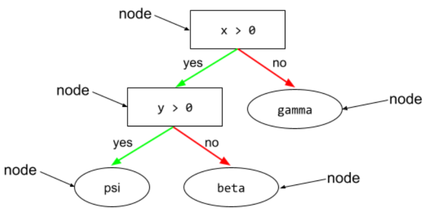
In a decision tree, any node that performs a test. For example, the following decision tree contains two conditions:
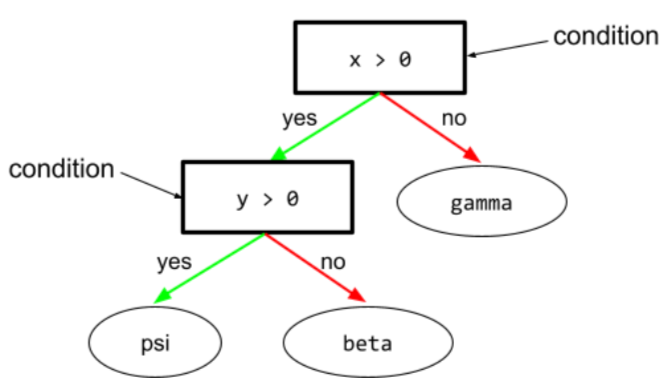
A condition is also called a split or a test.
Contrast condition with leaf.
See also:
See Types of conditions in the Decision Forests course for more information.
D
decision forest
A model created from multiple decision trees. A decision forest makes a prediction by aggregating the predictions of its decision trees. Popular types of decision forests include random forests and gradient boosted trees.
See the Decision Forests section in the Decision Forests course for more information.
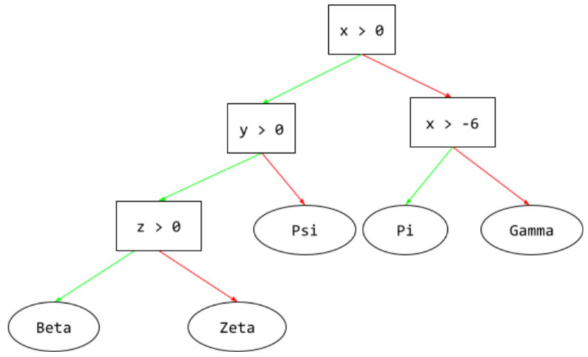
decision tree
A supervised learning model composed of a set of conditions and leaves organized hierarchically. For example, the following is a decision tree:
E
entropy
In information theory, a description of how unpredictable a probability distribution is. Alternatively, entropy is also defined as how much information each example contains. A distribution has the highest possible entropy when all values of a random variable are equally likely.
The entropy of a set with two possible values "0" and "1" (for example, the labels in a binary classification problem) has the following formula:
H = -p log p - q log q = -p log p - (1-p) * log (1-p)
where:
- H is the entropy.
- p is the fraction of "1" examples.
- q is the fraction of "0" examples. Note that q = (1 - p)
- log is generally log2. In this case, the entropy unit is a bit.
For example, suppose the following:
- 100 examples contain the value "1"
- 300 examples contain the value "0"
Therefore, the entropy value is:
- p = 0.25
- q = 0.75
- H = (-0.25)log2(0.25) - (0.75)log2(0.75) = 0.81 bits per example
A set that is perfectly balanced (for example, 200 "0"s and 200 "1"s) would have an entropy of 1.0 bit per example. As a set becomes more imbalanced, its entropy moves towards 0.0.
In decision trees, entropy helps formulate information gain to help the splitter select the conditions during the growth of a classification decision tree.
Compare entropy with:
- gini impurity
- cross-entropy loss function
Entropy is often called Shannon's entropy.
See Exact splitter for binary classification with numerical features in the Decision Forests course for more information.
F
feature importances
Synonym for variable importances.
G
gini impurity
A metric similar to entropy. Splitters use values derived from either gini impurity or entropy to compose conditions for classification decision trees. Information gain is derived from entropy. No universally accepted equivalent term for the metric derived from gini impurity exists; however, this unnamed metric is just as important as information gain.
Gini impurity is also called gini index, or simply gini.
gradient boosted (decision) trees (GBT)
A type of decision forest in which:
- Training relies on gradient boosting.
- The weak model is a decision tree.
See Gradient Boosted Decision Trees in the Decision Forests course for more information.
gradient boosting
A training algorithm where weak models are trained to iteratively improve the quality (reduce the loss) of a strong model. For example, a weak model could be a linear or small decision tree model. The strong model becomes the sum of all the previously trained weak models.
In the simplest form of gradient boosting, at each iteration, a weak model is trained to predict the loss gradient of the strong model. Then, the strong model's output is updated by subtracting the predicted gradient, similar to gradient descent.
where:
- $F_{0}$ is the starting strong model.
- $F_{i+1}$ is the next strong model.
- $F_{i}$ is the current strong model.
- $\xi$ is a value between 0.0 and 1.0 called shrinkage, which is analogous to the learning rate in gradient descent.
- $f_{i}$ is the weak model trained to predict the loss gradient of $F_{i}$.
Modern variations of gradient boosting also include the second derivative (Hessian) of the loss in their computation.
Decision trees are commonly used as weak models in gradient boosting. See gradient boosted (decision) trees.
I
inference path
In a decision tree, during inference, the route a particular example takes from the root to other conditions, terminating with a leaf. For example, in the following decision tree, the thicker arrows show the inference path for an example with the following feature values:
- x = 7
- y = 12
- z = -3
The inference path in the following illustration travels through three
conditions before reaching the leaf (Zeta).
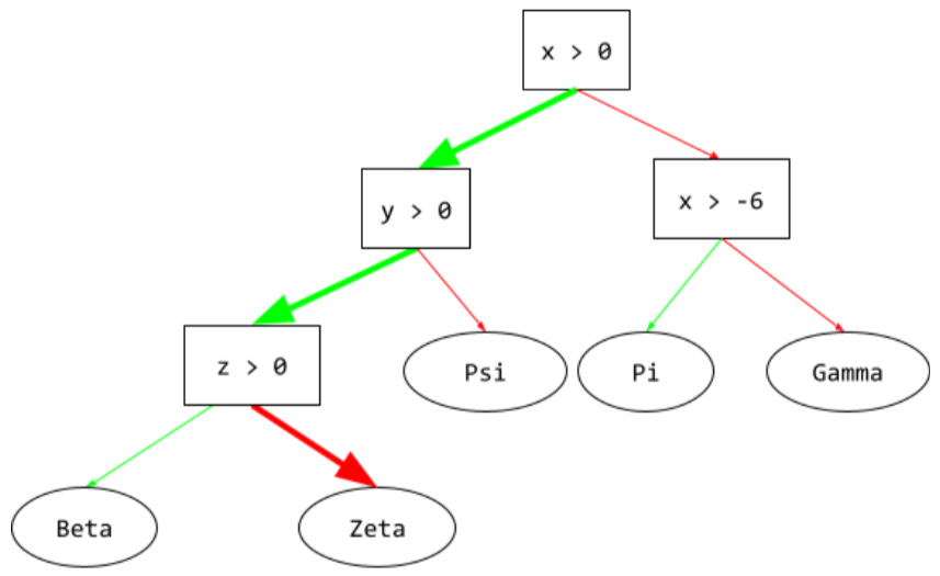
The three thick arrows show the inference path.
See Decision trees in the Decision Forests course for more information.
information gain
In decision forests, the difference between a node's entropy and the weighted (by number of examples) sum of the entropy of its children nodes. A node's entropy is the entropy of the examples in that node.
For example, consider the following entropy values:
- entropy of parent node = 0.6
- entropy of one child node with 16 relevant examples = 0.2
- entropy of another child node with 24 relevant examples = 0.1
So 40% of the examples are in one child node and 60% are in the other child node. Therefore:
- weighted entropy sum of child nodes = (0.4 * 0.2) + (0.6 * 0.1) = 0.14
So, the information gain is:
- information gain = entropy of parent node - weighted entropy sum of child nodes
- information gain = 0.6 - 0.14 = 0.46
Most splitters seek to create conditions that maximize information gain.
in-set condition
In a decision tree, a condition that tests for the presence of one item in a set of items. For example, the following is an in-set condition:
house-style in [tudor, colonial, cape]
During inference, if the value of the house-style feature
is tudor or colonial or cape, then this condition evaluates to Yes. If
the value of the house-style feature is something else (for example, ranch),
then this condition evaluates to No.
In-set conditions usually lead to more efficient decision trees than conditions that test one-hot encoded features.
L
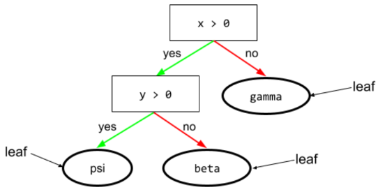
leaf
Any endpoint in a decision tree. Unlike a condition, a leaf doesn't perform a test. Rather, a leaf is a possible prediction. A leaf is also the terminal node of an inference path.
For example, the following decision tree contains three leaves:
See Decision trees in the Decision Forests course for more information.
N
node (decision tree)
In a decision tree, any condition or leaf.
See Decision Trees in the Decision Forests course for more information.
non-binary condition
A condition containing more than two possible outcomes. For example, the following non-binary condition contains three possible outcomes:
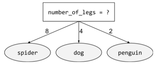
See Types of conditions in the Decision Forests course for more information.
O
oblique condition
In a decision tree, a condition that involves more than one feature. For example, if height and width are both features, then the following is an oblique condition:
height > width
Contrast with axis-aligned condition.
See Types of conditions in the Decision Forests course for more information.
out-of-bag evaluation (OOB evaluation)
A mechanism for evaluating the quality of a decision forest by testing each decision tree against the examples not used during training of that decision tree. For example, in the following diagram, notice that the system trains each decision tree on about two-thirds of the examples and then evaluates against the remaining one-third of the examples.
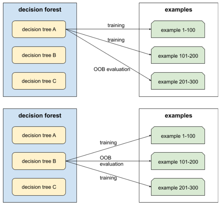
Out-of-bag evaluation is a computationally efficient and conservative approximation of the cross-validation mechanism. In cross-validation, one model is trained for each cross-validation round (for example, 10 models are trained in a 10-fold cross-validation). With OOB evaluation, a single model is trained. Because bagging withholds some data from each tree during training, OOB evaluation can use that data to approximate cross-validation.
See Out-of-bag evaluation in the Decision Forests course for more information.
P
permutation variable importances
A type of variable importance that evaluates the increase in the prediction error of a model after permuting the feature's values. Permutation variable importance is a model-independent metric.
R
random forest
An ensemble of decision trees in which each decision tree is trained with a specific random noise, such as bagging.
Random forests are a type of decision forest.
See Random Forest in the Decision Forests course for more information.
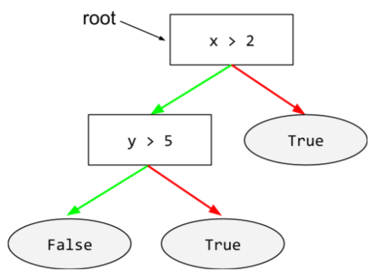
root
The starting node (the first condition) in a decision tree. By convention, diagrams put the root at the top of the decision tree. For example:
S
sampling with replacement
A method of picking items from a set of candidate items in which the same item can be picked multiple times. The phrase "with replacement" means that after each selection, the selected item is returned to the pool of candidate items. The inverse method, sampling without replacement, means that a candidate item can only be picked once.
For example, consider the following fruit set:
fruit = {kiwi, apple, pear, fig, cherry, lime, mango}Suppose that the system randomly picks fig as the first item.
If using sampling with replacement, then the system picks the
second item from the following set:
fruit = {kiwi, apple, pear, fig, cherry, lime, mango}Yes, that's the same set as before, so the system could potentially
pick fig again.
If using sampling without replacement, once picked, a sample can't be
picked again. For example, if the system randomly picks fig as the
first sample, then fig can't be picked again. Therefore, the system
picks the second sample from the following (reduced) set:
fruit = {kiwi, apple, pear, cherry, lime, mango}shrinkage
A hyperparameter in gradient boosting that controls overfitting. Shrinkage in gradient boosting is analogous to learning rate in gradient descent. Shrinkage is a decimal value between 0.0 and 1.0. A lower shrinkage value reduces overfitting more than a larger shrinkage value.
split
In a decision tree, another name for a condition.
splitter
While training a decision tree, the routine (and algorithm) responsible for finding the best condition at each node.
T
test
In a decision tree, another name for a condition.
threshold (for decision trees)
In an axis-aligned condition, the value that a feature is being compared against. For example, 75 is the threshold value in the following condition:
grade >= 75
See Exact splitter for binary classification with numerical features in the Decision Forests course for more information.
V
variable importances
A set of scores that indicates the relative importance of each feature to the model.
For example, consider a decision tree that estimates house prices. Suppose this decision tree uses three features: size, age, and style. If a set of variable importances for the three features are calculated to be {size=5.8, age=2.5, style=4.7}, then size is more important to the decision tree than age or style.
Different variable importance metrics exist, which can inform ML experts about different aspects of models.
W
wisdom of the crowd
The idea that averaging the opinions or estimates of a large group of people ("the crowd") often produces surprisingly good results. For example, consider a game in which people guess the number of jelly beans packed into a large jar. Although most individual guesses will be inaccurate, the average of all the guesses has been empirically shown to be surprisingly close to the actual number of jelly beans in the jar.
Ensembles are a software analog of wisdom of the crowd. Even if individual models make wildly inaccurate predictions, averaging the predictions of many models often generates surprisingly good predictions. For example, although an individual decision tree might make poor predictions, a decision forest often makes very good predictions.