

В Earth Engine есть несколько методов выполнения линейной регрессии с использованием редукторов:
ee.Reducer.linearFit()ee.Reducer.linearRegression()ee.Reducer.robustLinearRegression()ee.Reducer.ridgeRegression()
Простейший редуктор линейной регрессии – linearFit(), который вычисляет оценку линейной функции одной переменной с постоянным членом по методу наименьших квадратов. Для более гибкого подхода к линейному моделированию используйте один из редукторов линейной регрессии, которые позволяют использовать переменное число независимых и зависимых переменных. linearRegression() реализует обычную регрессию по методу наименьших квадратов(OLS). robustLinearRegression() использует функцию стоимости на основе остатков регрессии, чтобы итеративно снижать вес выбросов в данных (O’Leary, 1990).
ridgeRegression() выполняет линейную регрессию с регуляризацией L2.
Регрессионный анализ с использованием этих методов подходит для уменьшения объектов ee.ImageCollection, ee.Image, ee.FeatureCollection и ee.List.
Ниже приведены примеры использования каждого из них. Обратите внимание, что у функций linearRegression(), robustLinearRegression() и ridgeRegression() одинаковые структуры входных и выходных данных, но linearFit() ожидает двухдиапазонные входные данные (X, а затем Y), а у ridgeRegression() есть дополнительный параметр (lambda, необязательный) и выходные данные (pValue).
ee.ImageCollection
linearFit()
Данные должны быть настроены как двухполосное входное изображение, где первая полоса – это независимая переменная, а вторая – зависимая. В примере ниже показана оценка линейного тренда будущих осадков (после 2006 года в данных NEX-DCP30), спрогнозированных климатическими моделями. Зависимая переменная – прогнозируемые осадки, а независимая – время, добавленное перед вызовом linearFit():
Редактор кода (JavaScript)
// This function adds a time band to the image.
var createTimeBand = function(image) {
  // Scale milliseconds by a large constant to avoid very small slopes
  // in the linear regression output.
  return image.addBands(image.metadata('system:time_start').divide(1e18));
};

// Load the input image collection: projected climate data.
var collection = ee.ImageCollection('NASA/NEX-DCP30_ENSEMBLE_STATS')
  .filter(ee.Filter.eq('scenario', 'rcp85'))
  .filterDate(ee.Date('2006-01-01'), ee.Date('2050-01-01'))
  // Map the time band function over the collection.
  .map(createTimeBand);

// Reduce the collection with the linear fit reducer.
// Independent variable are followed by dependent variables.
var linearFit = collection.select(['system:time_start', 'pr_mean'])
  .reduce(ee.Reducer.linearFit());

// Display the results.
Map.setCenter(-100.11, 40.38, 5);
Map.addLayer(linearFit,
  {min: 0, max: [-0.9, 8e-5, 1], bands: ['scale', 'offset', 'scale']}, 'fit');
Обратите внимание, что выходные данные содержат две полосы: "смещение" (перехват) и "масштаб" ("масштаб" в этом контексте относится к наклону линии и его не следует путать с входным параметром масштаба для многих редукторов, который является пространственным масштабом). Результат, в котором области с возрастающим трендом выделены синим цветом, с убывающим – красным, а без тренда – зеленым, должен выглядеть примерно так, как показано на рисунке 1.
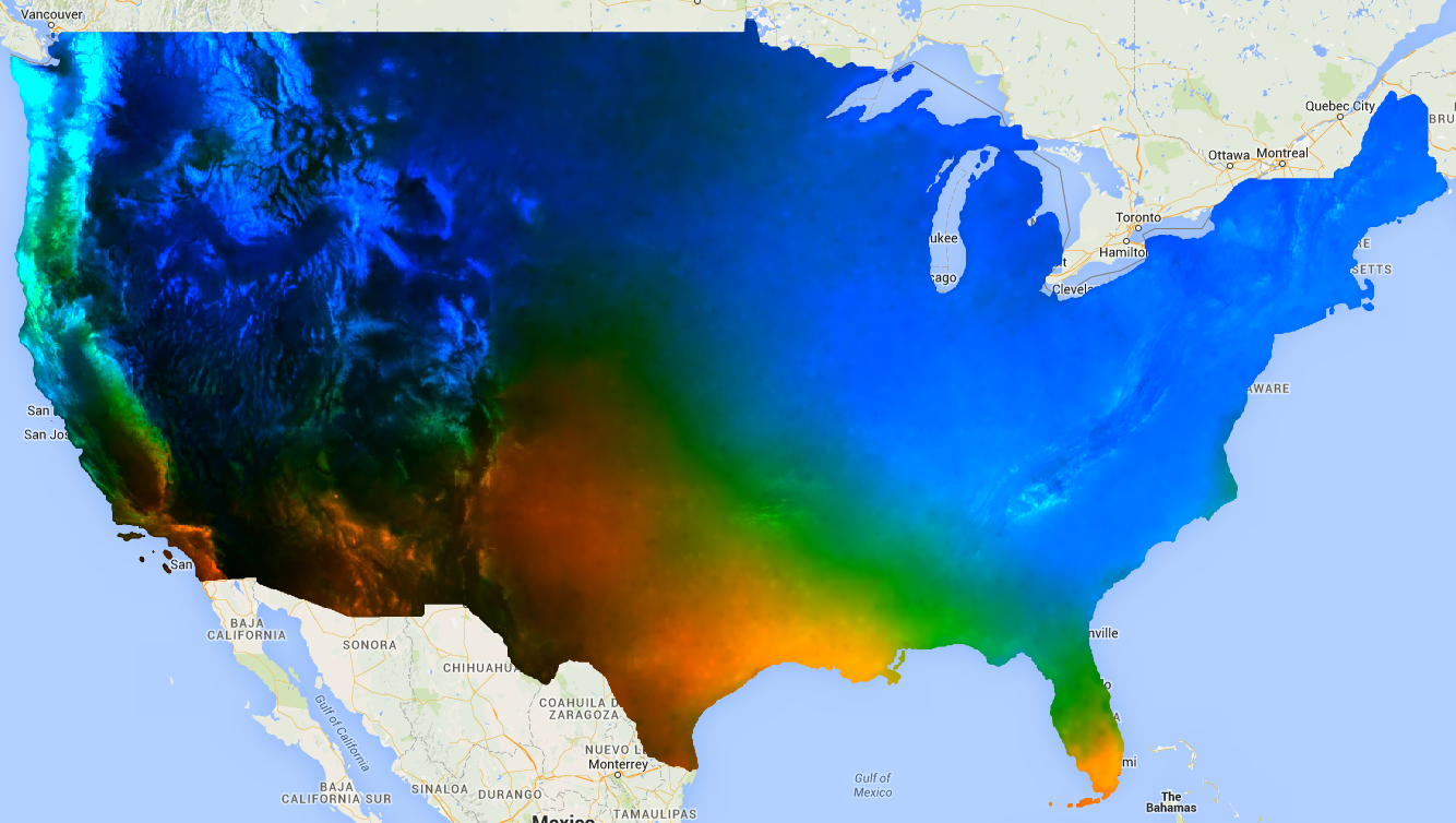
Рисунок 1. Результат linearFit(), примененный к прогнозируемым осадкам. Области, в которых прогнозируется увеличение количества осадков, показаны синим цветом, а уменьшение – красным.
linearRegression()
Например, предположим, что есть две зависимые переменные: осадки и максимальная температура, и две независимые переменные: константа и время. Коллекция идентична предыдущему примеру, но перед сокращением необходимо вручную добавить постоянную полосу. Первые две полосы входных данных – это независимые переменные X, а следующие две – зависимые переменные Y. В этом примере сначала получите коэффициенты регрессии, а затем выровняйте изображение массива, чтобы извлечь интересующие полосы:
Редактор кода (JavaScript)
// This function adds a time band to the image.
var createTimeBand = function(image) {
  // Scale milliseconds by a large constant.
  return image.addBands(image.metadata('system:time_start').divide(1e18));
};

// This function adds a constant band to the image.
var createConstantBand = function(image) {
  return ee.Image(1).addBands(image);
};

// Load the input image collection: projected climate data.
var collection = ee.ImageCollection('NASA/NEX-DCP30_ENSEMBLE_STATS')
  .filterDate(ee.Date('2006-01-01'), ee.Date('2099-01-01'))
  .filter(ee.Filter.eq('scenario', 'rcp85'))
  // Map the functions over the collection, to get constant and time bands.
  .map(createTimeBand)
  .map(createConstantBand)
  // Select the predictors and the responses.
  .select(['constant', 'system:time_start', 'pr_mean', 'tasmax_mean']);

// Compute ordinary least squares regression coefficients.
var linearRegression = collection.reduce(
  ee.Reducer.linearRegression({
    numX: 2,
    numY: 2
}));

// Compute robust linear regression coefficients.
var robustLinearRegression = collection.reduce(
  ee.Reducer.robustLinearRegression({
    numX: 2,
    numY: 2
}));

// The results are array images that must be flattened for display.
// These lists label the information along each axis of the arrays.
var bandNames = [['constant', 'time'], // 0-axis variation.
                 ['precip', 'temp']]; // 1-axis variation.

// Flatten the array images to get multi-band images according to the labels.
var lrImage = linearRegression.select(['coefficients']).arrayFlatten(bandNames);
var rlrImage = robustLinearRegression.select(['coefficients']).arrayFlatten(bandNames);

// Display the OLS results.
Map.setCenter(-100.11, 40.38, 5);
Map.addLayer(lrImage,
  {min: 0, max: [-0.9, 8e-5, 1], bands: ['time_precip', 'constant_precip', 'time_precip']}, 'OLS');

// Compare the results at a specific point:
print('OLS estimates:', lrImage.reduceRegion({
  reducer: ee.Reducer.first(),
  geometry: ee.Geometry.Point([-96.0, 41.0]),
  scale: 1000
}));

print('Robust estimates:', rlrImage.reduceRegion({
  reducer: ee.Reducer.first(),
  geometry: ee.Geometry.Point([-96.0, 41.0]),
  scale: 1000
}));
Проверьте результаты, чтобы убедиться, что выходные данные linearRegression() эквивалентны коэффициентам, рассчитанным редуктором linearFit(), хотя выходные данные linearRegression() также имеют коэффициенты для другой зависимой переменной, tasmax_mean. Коэффициенты робастной линейной регрессии отличаются от оценок МНК. В примере сравниваются коэффициенты, полученные с помощью разных методов регрессии в определенной точке.
ee.Image
В контексте объекта ee.Image редукторы регрессии можно использовать с reduceRegion или reduceRegions для выполнения линейной регрессии пикселей в регионе или регионах. В следующих примерах показано, как рассчитать коэффициенты регрессии между диапазонами Landsat в произвольном многоугольнике.
linearFit()
В разделе руководства, посвященном диаграммам на основе массивов данных, показана точечная диаграмма корреляции между диапазонами SWIR1 и SWIR2 Landsat 8. Здесь рассчитываются коэффициенты линейной регрессии для этой взаимосвязи. Возвращается словарь, содержащий свойства 'offset' (пересечение с осью Y) и 'scale' (наклон).
Редактор кода (JavaScript)
// Define a rectangle geometry around San Francisco.
var sanFrancisco = ee.Geometry.Rectangle([-122.45, 37.74, -122.4, 37.8]);

// Import a Landsat 8 TOA image for this region.
var img = ee.Image('LANDSAT/LC08/C02/T1_TOA/LC08_044034_20140318');

// Subset the SWIR1 and SWIR2 bands. In the regression reducer, independent
// variables come first followed by the dependent variables. In this case,
// B5 (SWIR1) is the independent variable and B6 (SWIR2) is the dependent
// variable.
var imgRegress = img.select(['B5', 'B6']);

// Calculate regression coefficients for the set of pixels intersecting the
// above defined region using reduceRegion with ee.Reducer.linearFit().
var linearFit = imgRegress.reduceRegion({
  reducer: ee.Reducer.linearFit(),
  geometry: sanFrancisco,
  scale: 30,
});

// Inspect the results.
print('OLS estimates:', linearFit);
print('y-intercept:', linearFit.get('offset'));
print('Slope:', linearFit.get('scale'));
linearRegression()
Здесь применяется тот же анализ, что и в предыдущем разделе linearFit, но на этот раз используется функция ee.Reducer.linearRegression. Обратите внимание, что регрессионное изображение состоит из трех отдельных изображений: постоянного изображения и изображений, представляющих полосы SWIR1 и SWIR2 из одного и того же изображения Landsat 8. Помните, что вы можете комбинировать любой набор полос для создания входного изображения для уменьшения региона с помощью ee.Reducer.linearRegression, они не обязательно должны принадлежать к одному и тому же исходному изображению.
Редактор кода (JavaScript)
// Define a rectangle geometry around San Francisco.
var sanFrancisco = ee.Geometry.Rectangle([-122.45, 37.74, -122.4, 37.8]);

// Import a Landsat 8 TOA image for this region.
var img = ee.Image('LANDSAT/LC08/C02/T1_TOA/LC08_044034_20140318');

// Create a new image that is the concatenation of three images: a constant,
// the SWIR1 band, and the SWIR2 band.
var constant = ee.Image(1);
var xVar = img.select('B5');
var yVar = img.select('B6');
var imgRegress = ee.Image.cat(constant, xVar, yVar);

// Calculate regression coefficients for the set of pixels intersecting the
// above defined region using reduceRegion. The numX parameter is set as 2
// because the constant and the SWIR1 bands are independent variables and they
// are the first two bands in the stack; numY is set as 1 because there is only
// one dependent variable (SWIR2) and it follows as band three in the stack.
var linearRegression = imgRegress.reduceRegion({
  reducer: ee.Reducer.linearRegression({
    numX: 2,
    numY: 1
  }),
  geometry: sanFrancisco,
  scale: 30,
});

// Convert the coefficients array to a list.
var coefList = ee.Array(linearRegression.get('coefficients')).toList();

// Extract the y-intercept and slope.
var b0 = ee.List(coefList.get(0)).get(0); // y-intercept
var b1 = ee.List(coefList.get(1)).get(0); // slope

// Extract the residuals.
var residuals = ee.Array(linearRegression.get('residuals')).toList().get(0);

// Inspect the results.
print('OLS estimates', linearRegression);
print('y-intercept:', b0);
print('Slope:', b1);
print('Residuals:', residuals);
Возвращается словарь, содержащий свойства 'coefficients' и 'residuals'. Свойство 'coefficients' – это массив с размерами (numX, numY). Каждый столбец содержит коэффициенты для соответствующей зависимой переменной. В данном случае массив состоит из двух строк и одного столбца. В первой строке первого столбца находится точка пересечения с осью Y, а во второй строке первого столбца – наклон. Свойство 'residuals' – это вектор среднеквадратичного значения остатков каждой зависимой переменной. Извлеките коэффициенты, преобразовав результат в массив и вырезав нужные элементы или преобразовав массив в список и выбрав коэффициенты по позиции индекса.
ee.FeatureCollection
Предположим, вы хотите узнать линейную зависимость между отражательной способностью Sentinel-2 и Landsat 8 SWIR1. В этом примере для расчета взаимосвязи используется случайная выборка пикселей, отформатированная как набор точек. Создается точечная диаграмма пар пикселей вместе с линией наилучшего соответствия по методу наименьших квадратов (рис. 2).
Редактор кода (JavaScript)
// Import a Sentinel-2 TOA image.
var s2ImgSwir1 = ee.Image('COPERNICUS/S2_HARMONIZED/20191022T185429_20191022T185427_T10SEH');

// Import a Landsat 8 TOA image from 12 days earlier than the S2 image.
var l8ImgSwir1 = ee.Image('LANDSAT/LC08/C02/T1_TOA/LC08_044033_20191010');

// Get the intersection between the two images - the area of interest (aoi).
var aoi = s2ImgSwir1.geometry().intersection(l8ImgSwir1.geometry());

// Get a set of 1000 random points from within the aoi. A feature collection
// is returned.
var sample = ee.FeatureCollection.randomPoints({
  region: aoi,
  points: 1000
});

// Combine the SWIR1 bands from each image into a single image.
var swir1Bands = s2ImgSwir1.select('B11')
  .addBands(l8ImgSwir1.select('B6'))
  .rename(['s2_swir1', 'l8_swir1']);

// Sample the SWIR1 bands using the sample point feature collection.
var imgSamp = swir1Bands.sampleRegions({
  collection: sample,
  scale: 30
})
// Add a constant property to each feature to be used as an independent variable.
.map(function(feature) {
  return feature.set('constant', 1);
});

// Compute linear regression coefficients. numX is 2 because
// there are two independent variables: 'constant' and 's2_swir1'. numY is 1
// because there is a single dependent variable: 'l8_swir1'. Cast the resulting
// object to an ee.Dictionary for easy access to the properties.
var linearRegression = ee.Dictionary(imgSamp.reduceColumns({
  reducer: ee.Reducer.linearRegression({
    numX: 2,
    numY: 1
  }),
  selectors: ['constant', 's2_swir1', 'l8_swir1']
}));

// Convert the coefficients array to a list.
var coefList = ee.Array(linearRegression.get('coefficients')).toList();

// Extract the y-intercept and slope.
var yInt = ee.List(coefList.get(0)).get(0); // y-intercept
var slope = ee.List(coefList.get(1)).get(0); // slope

// Gather the SWIR1 values from the point sample into a list of lists.
var props = ee.List(['s2_swir1', 'l8_swir1']);
var regressionVarsList = ee.List(imgSamp.reduceColumns({
  reducer: ee.Reducer.toList().repeat(props.size()),
  selectors: props
}).get('list'));

// Convert regression x and y variable lists to an array - used later as input
// to ui.Chart.array.values for generating a scatter plot.
var x = ee.Array(ee.List(regressionVarsList.get(0)));
var y1 = ee.Array(ee.List(regressionVarsList.get(1)));

// Apply the line function defined by the slope and y-intercept of the
// regression to the x variable list to create an array that will represent
// the regression line in the scatter plot.
var y2 = ee.Array(ee.List(regressionVarsList.get(0)).map(function(x) {
  var y = ee.Number(x).multiply(slope).add(yInt);
  return y;
}));

// Concatenate the y variables (Landsat 8 SWIR1 and predicted y) into an array
// for input to ui.Chart.array.values for plotting a scatter plot.
var yArr = ee.Array.cat([y1, y2], 1);

// Make a scatter plot of the two SWIR1 bands for the point sample and include
// the least squares line of best fit through the data.
print(ui.Chart.array.values({
  array: yArr,
  axis: 0,
  xLabels: x})
  .setChartType('ScatterChart')
  .setOptions({
    legend: {position: 'none'},
    hAxis: {'title': 'Sentinel-2 SWIR1'},
    vAxis: {'title': 'Landsat 8 SWIR1'},
    series: {
      0: {
        pointSize: 0.2,
        dataOpacity: 0.5,
      },
      1: {
        pointSize: 0,
        lineWidth: 2,
      }
    }
  })
);
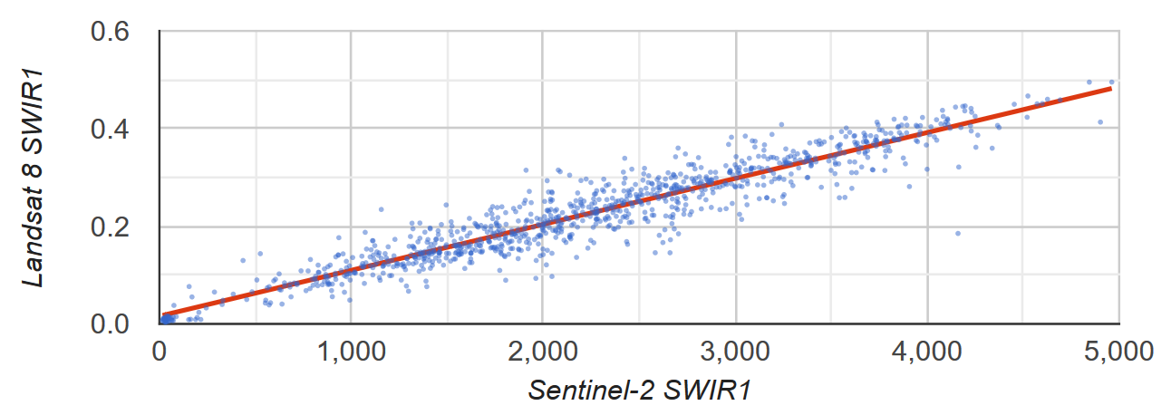
Рисунок 2. Точечная диаграмма и линия линейной регрессии по методу наименьших квадратов для выборки пикселей, представляющих отражательную способность Sentinel-2 и Landsat 8 SWIR1 TOA.
ee.List
Столбцы двумерных объектов ee.List могут быть входными данными для регрессионных редукторов. В примерах ниже приведены простые доказательства. Независимая переменная является копией зависимой переменной, в результате чего точка пересечения с осью Y равна 0, а наклон равен 1.
linearFit()
Редактор кода (JavaScript)
// Define a list of lists, where columns represent variables. The first column
// is the independent variable and the second is the dependent variable.
var listsVarColumns = ee.List([
  [1, 1],
  [2, 2],
  [3, 3],
  [4, 4],
  [5, 5]
]);

// Compute the least squares estimate of a linear function. Note that an
// object is returned; cast it as an ee.Dictionary to make accessing the
// coefficients easier.
var linearFit = ee.Dictionary(listsVarColumns.reduce(ee.Reducer.linearFit()));

// Inspect the result.
print(linearFit);
print('y-intercept:', linearFit.get('offset'));
print('Slope:', linearFit.get('scale'));
Транспонируйте список, если переменные представлены строками. Для этого преобразуйте его в ee.Array, транспонируйте, а затем преобразуйте обратно в ee.List.
Редактор кода (JavaScript)
// If variables in the list are arranged as rows, you'll need to transpose it.
// Define a list of lists where rows represent variables. The first row is the
// independent variable and the second is the dependent variable.
var listsVarRows = ee.List([
  [1, 2, 3, 4, 5],
  [1, 2, 3, 4, 5]
]);

// Cast the ee.List as an ee.Array, transpose it, and cast back to ee.List.
var listsVarColumns = ee.Array(listsVarRows).transpose().toList();

// Compute the least squares estimate of a linear function. Note that an
// object is returned; cast it as an ee.Dictionary to make accessing the
// coefficients easier.
var linearFit = ee.Dictionary(listsVarColumns.reduce(ee.Reducer.linearFit()));

// Inspect the result.
print(linearFit);
print('y-intercept:', linearFit.get('offset'));
print('Slope:', linearFit.get('scale'));
linearRegression()
Применение ee.Reducer.linearRegression() аналогично приведенному выше примеру linearFit(), за исключением того, что включена постоянная независимая переменная.
Редактор кода (JavaScript)
// Define a list of lists where columns represent variables. The first column
// represents a constant term, the second an independent variable, and the third
// a dependent variable.
var listsVarColumns = ee.List([
  [1, 1, 1],
  [1, 2, 2],
  [1, 3, 3],
  [1, 4, 4],
  [1, 5, 5]
]);

// Compute ordinary least squares regression coefficients. numX is 2 because
// there is one constant term and an additional independent variable. numY is 1
// because there is only a single dependent variable. Cast the resulting
// object to an ee.Dictionary for easy access to the properties.
var linearRegression = ee.Dictionary(
  listsVarColumns.reduce(ee.Reducer.linearRegression({
    numX: 2,
    numY: 1
})));

// Convert the coefficients array to a list.
var coefList = ee.Array(linearRegression.get('coefficients')).toList();

// Extract the y-intercept and slope.
var b0 = ee.List(coefList.get(0)).get(0); // y-intercept
var b1 = ee.List(coefList.get(1)).get(0); // slope

// Extract the residuals.
var residuals = ee.Array(linearRegression.get('residuals')).toList().get(0);

// Inspect the results.
print('OLS estimates', linearRegression);
print('y-intercept:', b0);
print('Slope:', b1);
print('Residuals:', residuals);