 GitHub에서 소스 보기
이미지 데이터의 RGB 시각적 표현을 생성하는 여러 ee.Image 메서드가 있습니다(예: visualize(), getThumbURL(), getMap(), getMapId()(Colab Folium 지도 표시에서 사용), Map.addLayer()(Code 편집기 지도 표시에서 사용, Python에서는 사용할 수 없음)). 기본적으로 이 메서드는 처음 세 개의 밴드를 각각 빨간색, 녹색, 파란색에 할당합니다. 기본 스트레치는 밴드의 데이터 유형에 따라 달라질 수 있습니다 (예: 부동 소수점은 [0, 1]에서 스트레칭되고 16비트 데이터는 가능한 모든 값 범위로 스트레칭됨). 원하는 시각화 효과를 얻으려면 시각화 매개변수를 제공하면 됩니다.
| 매개변수 | 설명 | 유형 |
|---|---|---|
| 밴드 | RGB에 매핑할 3개의 밴드 이름을 쉼표로 구분한 목록입니다. | list |
| min | 0으로 매핑할 값 | 밴드별로 하나씩 세 개의 숫자 또는 숫자 목록 |
| max | 255에 매핑할 값 | 3개의 숫자(밴드당 1개) 또는 숫자 목록 |
| gain | 각 픽셀 값에 곱할 값 | 3개의 숫자(밴드당 1개) 또는 숫자 목록 |
| bias | 각 DN에 추가할 값 | 3개의 숫자(밴드당 1개) 또는 숫자 목록 |
| gamma | 감마 보정 계수 | 3개의 숫자(밴드당 1개) 또는 숫자 목록 |
| palette | CSS 스타일 색상 문자열 목록 (단일 밴드 이미지만 해당) | 쉼표로 구분된 16진수 문자열 목록 |
| opacity | 레이어의 불투명도입니다 (0.0은 완전히 투명하고 1.0은 완전히 불투명함). | 숫자 |
| 형식 | 'jpg' 또는 'png' | 문자열 |
RGB 합성물
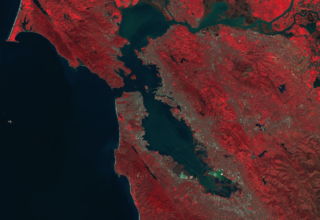
다음은 매개변수를 사용하여 Landsat 8 이미지의 스타일을 가짜 컬러 합성으로 지정하는 방법을 보여줍니다.
코드 편집기 (JavaScript)
// Load an image.
var image = ee.Image('LANDSAT/LC08/C02/T1_TOA/LC08_044034_20140318');

// Define the visualization parameters.
var vizParams = {
  bands: ['B5', 'B4', 'B3'],
  min: 0,
  max: 0.5,
  gamma: [0.95, 1.1, 1]
};

// Center the map and display the image.
Map.setCenter(-122.1899, 37.5010, 10); // San Francisco Bay
Map.addLayer(image, vizParams, 'false color composite');
import ee
import geemap.core as geemap
Colab (Python)
# Load an image.
image = ee.Image('LANDSAT/LC08/C02/T1_TOA/LC08_044034_20140318')

# Define the visualization parameters.
image_viz_params = {
    'bands': ['B5', 'B4', 'B3'],
    'min': 0,
    'max': 0.5,
    'gamma': [0.95, 1.1, 1],
}

# Define a map centered on San Francisco Bay.
map_l8 = geemap.Map(center=[37.5010, -122.1899], zoom=10)

# Add the image layer to the map and display it.
map_l8.add_layer(image, image_viz_params, 'false color composite')
display(map_l8)
이 예에서 밴드 'B5'는 빨간색에, 'B4'는 녹색에, 'B3'는 파란색에 할당됩니다.
색상 팔레트
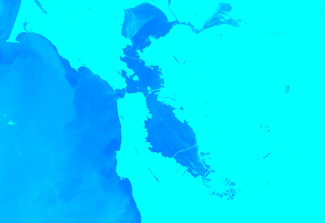
이미지의 단일 밴드를 색상으로 표시하려면 CSS 스타일 색상 문자열 목록으로 표현된 색상 램프로 palette 매개변수를 설정합니다. 자세한 내용은 이 참조를 참고하세요. 다음 예는 청록색('00FFFF')에서 파란색 ('0000FF')까지의 색상을 사용하여
정규화된 물 차이 지수 (NDWI) 이미지를 렌더링하는 방법을 보여줍니다.
코드 편집기 (JavaScript)
// Load an image.
var image = ee.Image('LANDSAT/LC08/C02/T1_TOA/LC08_044034_20140318');

// Create an NDWI image, define visualization parameters and display.
var ndwi = image.normalizedDifference(['B3', 'B5']);
var ndwiViz = {min: 0.5, max: 1, palette: ['00FFFF', '0000FF']};
Map.addLayer(ndwi, ndwiViz, 'NDWI', false);
import ee
import geemap.core as geemap
Colab (Python)
# Load an image.
image = ee.Image('LANDSAT/LC08/C02/T1_TOA/LC08_044034_20140318')

# Create an NDWI image, define visualization parameters and display.
ndwi = image.normalizedDifference(['B3', 'B5'])
ndwi_viz = {'min': 0.5, 'max': 1, 'palette': ['00FFFF', '0000FF']}

# Define a map centered on San Francisco Bay.
map_ndwi = geemap.Map(center=[37.5010, -122.1899], zoom=10)

# Add the image layer to the map and display it.
map_ndwi.add_layer(ndwi, ndwi_viz, 'NDWI')
display(map_ndwi)
이 예에서 min 및 max 매개변수는 팔레트를 적용할 픽셀 값의 범위를 나타냅니다. 중간 값은 선형으로 늘어납니다.
또한 코드 편집기 예시에서 show 매개변수가 false로 설정되어 있습니다. 이렇게 하면 레이어가 지도에 추가될 때 레이어의 공개 상태가 사용 중지됩니다. 코드 편집기 지도의 오른쪽 상단에 있는 레이어 관리자를 사용하여 언제든지 다시 사용 설정할 수 있습니다.
기본 색상 팔레트 저장
색상 팔레트를 적용하는 것을 잊지 않도록 분류 이미지에 색상 팔레트를 저장하려면 각 분류 밴드에 특별한 이름이 지정된 두 개의 문자열 이미지 속성을 설정하면 됩니다.
예를 들어 이미지에 'landcover'라는 밴드가 있고 'water', 'forest', 'other' 클래스에 해당하는 세 가지 값 0, 1, 2가 있는 경우 다음 속성을 설정하여 기본 시각화에서 각 클래스에 지정된 색상을 표시할 수 있습니다 (분석에 사용된 값은 영향을 받지 않음).
landcover_class_values="0,1,2"landcover_class_palette="0000FF,00FF00,AABBCD"
저작물 메타데이터를 설정하는 방법은 저작물 관리 페이지를 참고하세요.
마스킹
image.updateMask()를 사용하여 마스크 이미지의 픽셀이 0이 아닌 위치를 기반으로 개별 픽셀의 불투명도를 설정할 수 있습니다. 마스크에서 0과 같은 픽셀은 계산에서 제외되고 불투명도는 디스플레이용으로 0으로 설정됩니다. 다음 예에서는 NDWI 임곗값 (임곗값에 관한 정보는
연산 섹션 참고)을 사용하여 이전에 만든 NDWI 레이어의 마스크를 업데이트합니다.
코드 편집기 (JavaScript)
// Mask the non-watery parts of the image, where NDWI < 0.4.
var ndwiMasked = ndwi.updateMask(ndwi.gte(0.4));
Map.addLayer(ndwiMasked, ndwiViz, 'NDWI masked');
import ee
import geemap.core as geemap
Colab (Python)
# Mask the non-watery parts of the image, where NDWI < 0.4.
ndwi_masked = ndwi.updateMask(ndwi.gte(0.4))

# Define a map centered on San Francisco Bay.
map_ndwi_masked = geemap.Map(center=[37.5010, -122.1899], zoom=10)

# Add the image layer to the map and display it.
map_ndwi_masked.add_layer(ndwi_masked, ndwi_viz, 'NDWI masked')
display(map_ndwi_masked)
시각화 이미지
image.visualize() 메서드를 사용하여 이미지를 8비트 RGB 이미지로 변환하여 표시하거나 내보냅니다. 예를 들어 가상 색상 합성물과 NDWI를 3밴드 디스플레이 이미지로 변환하려면 다음을 사용하세요.
코드 편집기 (JavaScript)
// Create visualization layers.
var imageRGB = image.visualize({bands: ['B5', 'B4', 'B3'], max: 0.5});
var ndwiRGB = ndwiMasked.visualize({
  min: 0.5,
  max: 1,
  palette: ['00FFFF', '0000FF']
});
import ee
import geemap.core as geemap
Colab (Python)
image_rgb = image.visualize(bands=['B5', 'B4', 'B3'], max=0.5)
ndwi_rgb = ndwi_masked.visualize(min=0.5, max=1, palette=['00FFFF', '0000FF'])
모자이크 처리
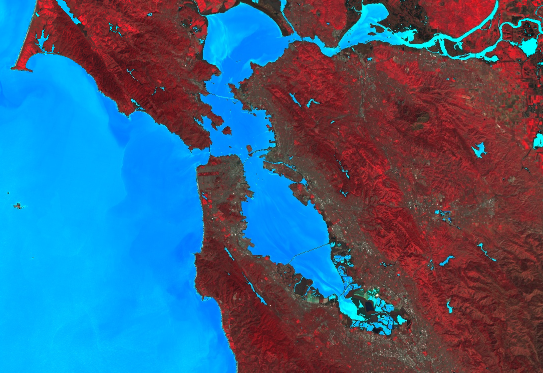
마스킹 및 imageCollection.mosaic() (모자이크에 관한 정보는 모자이크 섹션 참고)를 사용하여 다양한 지리 정보 효과를 얻을 수 있습니다. mosaic() 메서드는 입력 컬렉션의 순서에 따라 출력 이미지의 레이어를 렌더링합니다. 다음 예에서는 mosaic()를 사용하여 마스크된 NDWI와 가짜 컬러 합성물을 결합하고 새 시각화를 얻습니다.
코드 편집기 (JavaScript)
// Mosaic the visualization layers and display (or export).
var mosaic = ee.ImageCollection([imageRGB, ndwiRGB]).mosaic();
Map.addLayer(mosaic, {}, 'mosaic');
import ee
import geemap.core as geemap
Colab (Python)
# Mosaic the visualization layers and display (or export).
mosaic = ee.ImageCollection([image_rgb, ndwi_rgb]).mosaic()

# Define a map centered on San Francisco Bay.
map_mosaic = geemap.Map(center=[37.5010, -122.1899], zoom=10)

# Add the image layer to the map and display it.
map_mosaic.add_layer(mosaic, None, 'mosaic')
display(map_mosaic)
이 예에서는 두 시각화 이미지의 목록이 ImageCollection 생성자에 제공됩니다. 목록의 순서에 따라 지도에 이미지가 렌더링되는 순서가 결정됩니다.
클리핑
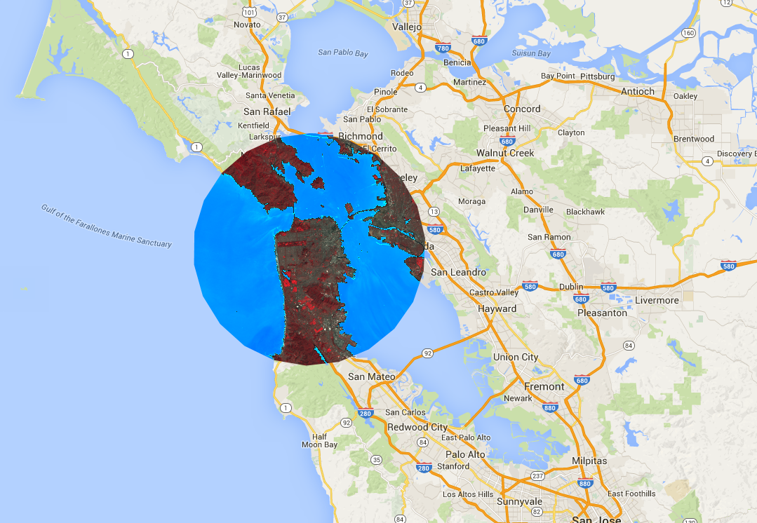
image.clip() 메서드는 지리 정보 효과를 얻는 데 유용합니다. 다음 예에서는 이전에 만든 모자이크를 샌프란시스코 시 주변의 임의 버퍼 영역으로 자릅니다.
코드 편집기 (JavaScript)
// Create a circle by drawing a 20000 meter buffer around a point.
var roi = ee.Geometry.Point([-122.4481, 37.7599]).buffer(20000);

// Display a clipped version of the mosaic.
Map.addLayer(mosaic.clip(roi), null, 'mosaic clipped');
import ee
import geemap.core as geemap
Colab (Python)
# Create a circle by drawing a 20000 meter buffer around a point.
roi = ee.Geometry.Point([-122.4481, 37.7599]).buffer(20000)
mosaic_clipped = mosaic.clip(roi)

# Define a map centered on San Francisco.
map_mosaic_clipped = geemap.Map(center=[37.7599, -122.4481], zoom=10)

# Add the image layer to the map and display it.
map_mosaic_clipped.add_layer(mosaic_clipped, None, 'mosaic clipped')
display(map_mosaic_clipped)
위 예에서 좌표는 Geometry 생성자에 제공되고 버퍼 길이는 20,000미터로 지정됩니다. 지오메트리 페이지에서 지오메트리에 대해 자세히 알아보세요.
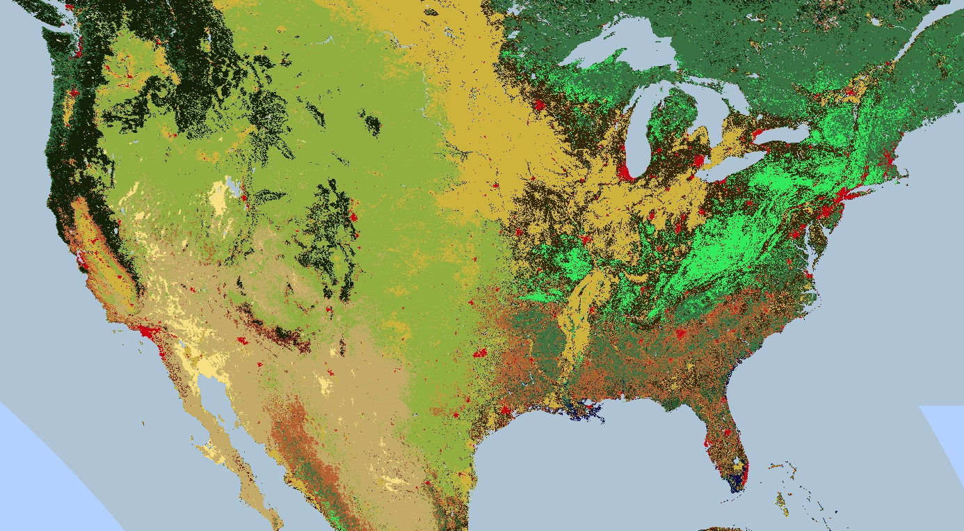
범주 지도 렌더링
팔레트는 토지 피복 지도와 같이 불연속 값 지도 렌더링에도 유용합니다.
클래스가 여러 개인 경우 팔레트를 사용하여 각 클래스에 다른 색상을 지정합니다.
이 맥락에서 임의의 라벨을 연속 정수로 변환하는 데 image.remap() 메서드가 유용할 수 있습니다. 다음 예에서는 팔레트를 사용하여 토지 피복 카테고리를 렌더링합니다.
코드 편집기 (JavaScript)
// Load 2012 MODIS land cover and select the IGBP classification.
var cover = ee.Image('MODIS/051/MCD12Q1/2012_01_01')
  .select('Land_Cover_Type_1');

// Define a palette for the 18 distinct land cover classes.
var igbpPalette = [
  'aec3d4', // water
  '152106', '225129', '369b47', '30eb5b', '387242', // forest
  '6a2325', 'c3aa69', 'b76031', 'd9903d', '91af40',  // shrub, grass
  '111149', // wetlands
  'cdb33b', // croplands
  'cc0013', // urban
  '33280d', // crop mosaic
  'd7cdcc', // snow and ice
  'f7e084', // barren
  '6f6f6f'  // tundra
];

// Specify the min and max labels and the color palette matching the labels.
Map.setCenter(-99.229, 40.413, 5);
Map.addLayer(cover,
             {min: 0, max: 17, palette: igbpPalette},
             'IGBP classification');
import ee
import geemap.core as geemap
Colab (Python)
# Load 2012 MODIS land cover and select the IGBP classification.
cover = ee.Image('MODIS/051/MCD12Q1/2012_01_01').select('Land_Cover_Type_1')

# Define a palette for the 18 distinct land cover classes.
igbp_palette = [
    'aec3d4',  # water
    '152106',
    '225129',
    '369b47',
    '30eb5b',
    '387242',  # forest
    '6a2325',
    'c3aa69',
    'b76031',
    'd9903d',
    '91af40',  # shrub, grass
    '111149',  # wetlands
    'cdb33b',  # croplands
    'cc0013',  # urban
    '33280d',  # crop mosaic
    'd7cdcc',  # snow and ice
    'f7e084',  # barren
    '6f6f6f',  # tundra
]

# Define a map centered on the United States.
map_palette = geemap.Map(center=[40.413, -99.229], zoom=5)

# Add the image layer to the map and display it. Specify the min and max labels
# and the color palette matching the labels.
map_palette.add_layer(
    cover, {'min': 0, 'max': 17, 'palette': igbp_palette}, 'IGBP classes'
)
display(map_palette)
스타일 지정된 레이어 설명자
스타일 지정된 레이어 설명자(SLD)를 사용하여 디스플레이용 이미지를 렌더링할 수 있습니다. image.sldStyle()에 이미지의 기호화 및 색상에 관한 XML 설명(특히 RasterSymbolizer 요소)을 제공합니다. RasterSymbolizer 요소에 관한 자세한 내용은 여기를 참고하세요.
예를 들어 카테고리 지도 렌더링 섹션에 설명된 토지 피복 지도를 SLD로 렌더링하려면 다음을 사용하세요.
코드 편집기 (JavaScript)
var cover = ee.Image('MODIS/051/MCD12Q1/2012_01_01').select('Land_Cover_Type_1');

// Define an SLD style of discrete intervals to apply to the image.
var sld_intervals =
'<RasterSymbolizer>' +
  '<ColorMap type="intervals" extended="false">' +
    '<ColorMapEntry color="#aec3d4" quantity="0" label="Water"/>' +
    '<ColorMapEntry color="#152106" quantity="1" label="Evergreen Needleleaf Forest"/>' +
    '<ColorMapEntry color="#225129" quantity="2" label="Evergreen Broadleaf Forest"/>' +
    '<ColorMapEntry color="#369b47" quantity="3" label="Deciduous Needleleaf Forest"/>' +
    '<ColorMapEntry color="#30eb5b" quantity="4" label="Deciduous Broadleaf Forest"/>' +
    '<ColorMapEntry color="#387242" quantity="5" label="Mixed Deciduous Forest"/>' +
    '<ColorMapEntry color="#6a2325" quantity="6" label="Closed Shrubland"/>' +
    '<ColorMapEntry color="#c3aa69" quantity="7" label="Open Shrubland"/>' +
    '<ColorMapEntry color="#b76031" quantity="8" label="Woody Savanna"/>' +
    '<ColorMapEntry color="#d9903d" quantity="9" label="Savanna"/>' +
    '<ColorMapEntry color="#91af40" quantity="10" label="Grassland"/>' +
    '<ColorMapEntry color="#111149" quantity="11" label="Permanent Wetland"/>' +
    '<ColorMapEntry color="#cdb33b" quantity="12" label="Cropland"/>' +
    '<ColorMapEntry color="#cc0013" quantity="13" label="Urban"/>' +
    '<ColorMapEntry color="#33280d" quantity="14" label="Crop, Natural Veg. Mosaic"/>' +
    '<ColorMapEntry color="#d7cdcc" quantity="15" label="Permanent Snow, Ice"/>' +
    '<ColorMapEntry color="#f7e084" quantity="16" label="Barren, Desert"/>' +
    '<ColorMapEntry color="#6f6f6f" quantity="17" label="Tundra"/>' +
  '</ColorMap>' +
'</RasterSymbolizer>';
Map.addLayer(cover.sldStyle(sld_intervals), {}, 'IGBP classification styled');
import ee
import geemap.core as geemap
Colab (Python)
cover = ee.Image('MODIS/051/MCD12Q1/2012_01_01').select('Land_Cover_Type_1')

# Define an SLD style of discrete intervals to apply to the image.
sld_intervals = """
<RasterSymbolizer>
  <ColorMap  type="intervals" extended="false" >
    <ColorMapEntry color="#aec3d4" quantity="0" label="Water"/>
    <ColorMapEntry color="#152106" quantity="1" label="Evergreen Needleleaf Forest"/>
    <ColorMapEntry color="#225129" quantity="2" label="Evergreen Broadleaf Forest"/>
    <ColorMapEntry color="#369b47" quantity="3" label="Deciduous Needleleaf Forest"/>
    <ColorMapEntry color="#30eb5b" quantity="4" label="Deciduous Broadleaf Forest"/>
    <ColorMapEntry color="#387242" quantity="5" label="Mixed Deciduous Forest"/>
    <ColorMapEntry color="#6a2325" quantity="6" label="Closed Shrubland"/>
    <ColorMapEntry color="#c3aa69" quantity="7" label="Open Shrubland"/>
    <ColorMapEntry color="#b76031" quantity="8" label="Woody Savanna"/>
    <ColorMapEntry color="#d9903d" quantity="9" label="Savanna"/>
    <ColorMapEntry color="#91af40" quantity="10" label="Grassland"/>
    <ColorMapEntry color="#111149" quantity="11" label="Permanent Wetland"/>
    <ColorMapEntry color="#cdb33b" quantity="12" label="Cropland"/>
    <ColorMapEntry color="#cc0013" quantity="13" label="Urban"/>
    <ColorMapEntry color="#33280d" quantity="14" label="Crop, Natural Veg. Mosaic"/>
    <ColorMapEntry color="#d7cdcc" quantity="15" label="Permanent Snow, Ice"/>
    <ColorMapEntry color="#f7e084" quantity="16" label="Barren, Desert"/>
    <ColorMapEntry color="#6f6f6f" quantity="17" label="Tundra"/>
  </ColorMap>
</RasterSymbolizer>"""

# Apply the SLD style to the image.
cover_sld = cover.sldStyle(sld_intervals)

# Define a map centered on the United States.
map_sld_categorical = geemap.Map(center=[40.413, -99.229], zoom=5)

# Add the image layer to the map and display it.
map_sld_categorical.add_layer(cover_sld, None, 'IGBP classes styled')
display(map_sld_categorical)
색상 범위가 있는 시각화 이미지를 만들려면 ColorMap의 유형을 'ramp'로 설정합니다. 다음 예에서는 DEM 렌더링을 위한 '간격' 및 '램프' 유형을 비교합니다.
코드 편집기 (JavaScript)
// Load SRTM Digital Elevation Model data.
var image = ee.Image('CGIAR/SRTM90_V4');

// Define an SLD style of discrete intervals to apply to the image. Use the
// opacity keyword to set pixels less than 0 as completely transparent. Pixels
// with values greater than or equal to the final entry quantity are set to
// fully transparent by default.
var sld_intervals =
  '<RasterSymbolizer>' +
    '<ColorMap type="intervals" extended="false" >' +
      '<ColorMapEntry color="#0000ff" quantity="0" label="0 ﹤ x" opacity="0" />' +
      '<ColorMapEntry color="#00ff00" quantity="100" label="0 ≤ x ﹤ 100" />' +
      '<ColorMapEntry color="#007f30" quantity="200" label="100 ≤ x ﹤ 200" />' +
      '<ColorMapEntry color="#30b855" quantity="300" label="200 ≤ x ﹤ 300" />' +
      '<ColorMapEntry color="#ff0000" quantity="400" label="300 ≤ x ﹤ 400" />' +
      '<ColorMapEntry color="#ffff00" quantity="900" label="400 ≤ x ﹤ 900" />' +
    '</ColorMap>' +
  '</RasterSymbolizer>';

// Define an sld style color ramp to apply to the image.
var sld_ramp =
  '<RasterSymbolizer>' +
    '<ColorMap type="ramp" extended="false" >' +
      '<ColorMapEntry color="#0000ff" quantity="0" label="0"/>' +
      '<ColorMapEntry color="#00ff00" quantity="100" label="100" />' +
      '<ColorMapEntry color="#007f30" quantity="200" label="200" />' +
      '<ColorMapEntry color="#30b855" quantity="300" label="300" />' +
      '<ColorMapEntry color="#ff0000" quantity="400" label="400" />' +
      '<ColorMapEntry color="#ffff00" quantity="500" label="500" />' +
    '</ColorMap>' +
  '</RasterSymbolizer>';

// Add the image to the map using both the color ramp and interval schemes.
Map.setCenter(-76.8054, 42.0289, 8);
Map.addLayer(image.sldStyle(sld_intervals), {}, 'SLD intervals');
Map.addLayer(image.sldStyle(sld_ramp), {}, 'SLD ramp');
import ee
import geemap.core as geemap
Colab (Python)
# Load SRTM Digital Elevation Model data.
image = ee.Image('CGIAR/SRTM90_V4')

# Define an SLD style of discrete intervals to apply to the image.
sld_intervals = """
    <RasterSymbolizer>
      <ColorMap type="intervals" extended="false" >
        <ColorMapEntry color="#0000ff" quantity="0" label="0"/>
        <ColorMapEntry color="#00ff00" quantity="100" label="1-100" />
        <ColorMapEntry color="#007f30" quantity="200" label="110-200" />
        <ColorMapEntry color="#30b855" quantity="300" label="210-300" />
        <ColorMapEntry color="#ff0000" quantity="400" label="310-400" />
        <ColorMapEntry color="#ffff00" quantity="1000" label="410-1000" />
      </ColorMap>
    </RasterSymbolizer>"""

# Define an sld style color ramp to apply to the image.
sld_ramp = """
    <RasterSymbolizer>
      <ColorMap type="ramp" extended="false" >
        <ColorMapEntry color="#0000ff" quantity="0" label="0"/>
        <ColorMapEntry color="#00ff00" quantity="100" label="100" />
        <ColorMapEntry color="#007f30" quantity="200" label="200" />
        <ColorMapEntry color="#30b855" quantity="300" label="300" />
        <ColorMapEntry color="#ff0000" quantity="400" label="400" />
        <ColorMapEntry color="#ffff00" quantity="500" label="500" />
      </ColorMap>
    </RasterSymbolizer>"""

# Define a map centered on the United States.
map_sld_interval = geemap.Map(center=[40.413, -99.229], zoom=5)

# Add the image layers to the map and display it.
map_sld_interval.add_layer(
    image.sldStyle(sld_intervals), None, 'SLD intervals'
)
map_sld_interval.add_layer(image.sldStyle(sld_ramp), None, 'SLD ramp')
display(map_sld_interval)
SLD는 연속 데이터의 시각화를 개선하기 위해 픽셀 값을 늘리는 데도 유용합니다. 예를 들어 다음 코드는 임의의 선형 스트레치 결과를 최솟값-최댓값 '정규화' 및 '히스토그램' 등화와 비교합니다.
코드 편집기 (JavaScript)
// Load a Landsat 8 raw image.
var image = ee.Image('LANDSAT/LC08/C02/T1/LC08_044034_20140318');

// Define a RasterSymbolizer element with '_enhance_' for a placeholder.
var template_sld =
  '<RasterSymbolizer>' +
    '<ContrastEnhancement><_enhance_/></ContrastEnhancement>' +
    '<ChannelSelection>' +
      '<RedChannel>' +
        '<SourceChannelName>B5</SourceChannelName>' +
      '</RedChannel>' +
      '<GreenChannel>' +
        '<SourceChannelName>B4</SourceChannelName>' +
      '</GreenChannel>' +
      '<BlueChannel>' +
        '<SourceChannelName>B3</SourceChannelName>' +
      '</BlueChannel>' +
    '</ChannelSelection>' +
  '</RasterSymbolizer>';

// Get SLDs with different enhancements.
var equalize_sld = template_sld.replace('_enhance_', 'Histogram');
var normalize_sld = template_sld.replace('_enhance_', 'Normalize');

// Display the results.
Map.centerObject(image, 10);
Map.addLayer(image, {bands: ['B5', 'B4', 'B3'], min: 0, max: 15000}, 'Linear');
Map.addLayer(image.sldStyle(equalize_sld), {}, 'Equalized');
Map.addLayer(image.sldStyle(normalize_sld), {}, 'Normalized');
import ee
import geemap.core as geemap
Colab (Python)
# Load a Landsat 8 raw image.
image = ee.Image('LANDSAT/LC08/C02/T1/LC08_044034_20140318')

# Define a RasterSymbolizer element with '_enhance_' for a placeholder.
template_sld = """
<RasterSymbolizer>
  <ContrastEnhancement><_enhance_/></ContrastEnhancement>
  <ChannelSelection>
    <RedChannel>
      <SourceChannelName>B5</SourceChannelName>
    </RedChannel>
    <GreenChannel>
      <SourceChannelName>B4</SourceChannelName>
    </GreenChannel>
    <BlueChannel>
      <SourceChannelName>B3</SourceChannelName>
    </BlueChannel>
  </ChannelSelection>
</RasterSymbolizer>"""

# Get SLDs with different enhancements.
equalize_sld = template_sld.replace('_enhance_', 'Histogram')
normalize_sld = template_sld.replace('_enhance_', 'Normalize')

# Define a map centered on San Francisco Bay.
map_sld_continuous = geemap.Map(center=[37.5010, -122.1899], zoom=10)

# Add the image layers to the map and display it.
map_sld_continuous.add_layer(
    image, {'bands': ['B5', 'B4', 'B3'], 'min': 0, 'max': 15000}, 'Linear'
)
map_sld_continuous.add_layer(image.sldStyle(equalize_sld), None, 'Equalized')
map_sld_continuous.add_layer(
    image.sldStyle(normalize_sld), None, 'Normalized'
)
display(map_sld_continuous)
Earth Engine에서 SLD를 사용하는 것과 관련하여 유의해야 할 사항은 다음과 같습니다.
- OGC SLD 1.0 및 OGC SE 1.1이 지원됩니다.
- 전달된 XML 문서는 전체 문서일 수도 있고 RasterSymbolizer 요소와 그 아래 요소만 있을 수도 있습니다.
- 밴드는 Earth Engine 이름 또는 색인 ('1', '2', ...)으로 선택할 수 있습니다.
- 히스토그램 및 대비 스트레치 정규화 메커니즘은 부동 점 이미지에는 지원되지 않습니다.
- 불투명도는 0.0 (투명)인 경우에만 고려됩니다. 불투명도 값이 0이 아니면 완전히 불투명하게 취급됩니다.
- OverlapBehavior 정의는 현재 무시됩니다.
- ShadedRelief 메커니즘은 현재 지원되지 않습니다.
- ImageOutline 메커니즘은 현재 지원되지 않습니다.
- Geometry 요소는 무시됩니다.
- 히스토그램 평등화 또는 정규화가 요청된 경우 출력 이미지에 histogram_bandname 메타데이터가 포함됩니다.
썸네일 이미지
ee.Image.getThumbURL() 메서드를 사용하여 ee.Image 객체의 PNG 또는 JPEG 썸네일 이미지를 생성합니다. getThumbURL() 호출로 끝나는 표현식의 결과를 출력하면 URL이 출력됩니다. URL을 방문하면 요청된 썸네일을 즉시 생성하도록 Earth Engine 서버가 설정됩니다. 처리가 완료되면 이미지가 브라우저에 표시됩니다. 이미지의 마우스 오른쪽 버튼 컨텍스트 메뉴에서 적절한 옵션을 선택하여 다운로드할 수 있습니다.
getThumbURL() 메서드에는 위의 시각화 매개변수 표에 설명된 매개변수가 포함됩니다.
또한 썸네일의 공간 범위, 크기, 디스플레이 투영을 제어하는 선택적 dimensions, region, crs 인수를 사용합니다.
| 매개변수 | 설명 | 유형 |
|---|---|---|
| dimensions | 썸네일 크기(픽셀 단위)입니다. 단일 정수가 제공되면 이미지의 더 큰 가로세로 비율 크기를 정의하고 더 작은 크기를 비례하여 조정합니다. 큰 이미지 가로세로 비율의 기본값은 512픽셀입니다. | 'WIDTHxHEIGHT' 형식의 단일 정수 또는 문자열 |
| region | 렌더링할 이미지의 지리적 영역입니다. 기본적으로 전체 이미지 또는 제공된 도형의 경계입니다. | GeoJSON 또는 선형 링을 정의하는 점 좌표 3개 이상의 2D 목록 |
| crs | 타겟 프로젝션(예: 'EPSG:3857') 기본값은 WGS84 ('EPSG:4326')입니다. | 문자열 |
| 형식 | 썸네일 형식을 PNG 또는 JPEG로 정의합니다. 기본 PNG 형식은 RGBA로 구현되며 여기서 알파 채널은 이미지의 mask()에 의해 정의된 유효한 픽셀과 잘못된 픽셀을 나타냅니다. 잘못된 픽셀은 투명합니다. 선택적 JPEG 형식은 RGB로 구현되며, 여기서 잘못된 이미지 픽셀은 RGB 채널 전체에 0으로 채워집니다.
|
문자열('png' 또는 'jpg') |
palette 인수가 제공되지 않으면 단일 밴드 이미지는 기본적으로 그레이스케일로 설정됩니다. bands 인수가 제공되지 않는 한 멀티밴드 이미지는 기본적으로 처음 세 밴드의 RGB 시각화로 설정됩니다. 두 개의 밴드만 제공되면 첫 번째 밴드는 빨간색에 매핑되고 두 번째 밴드는 파란색에 매핑되며 녹색 채널은 0으로 채워집니다.
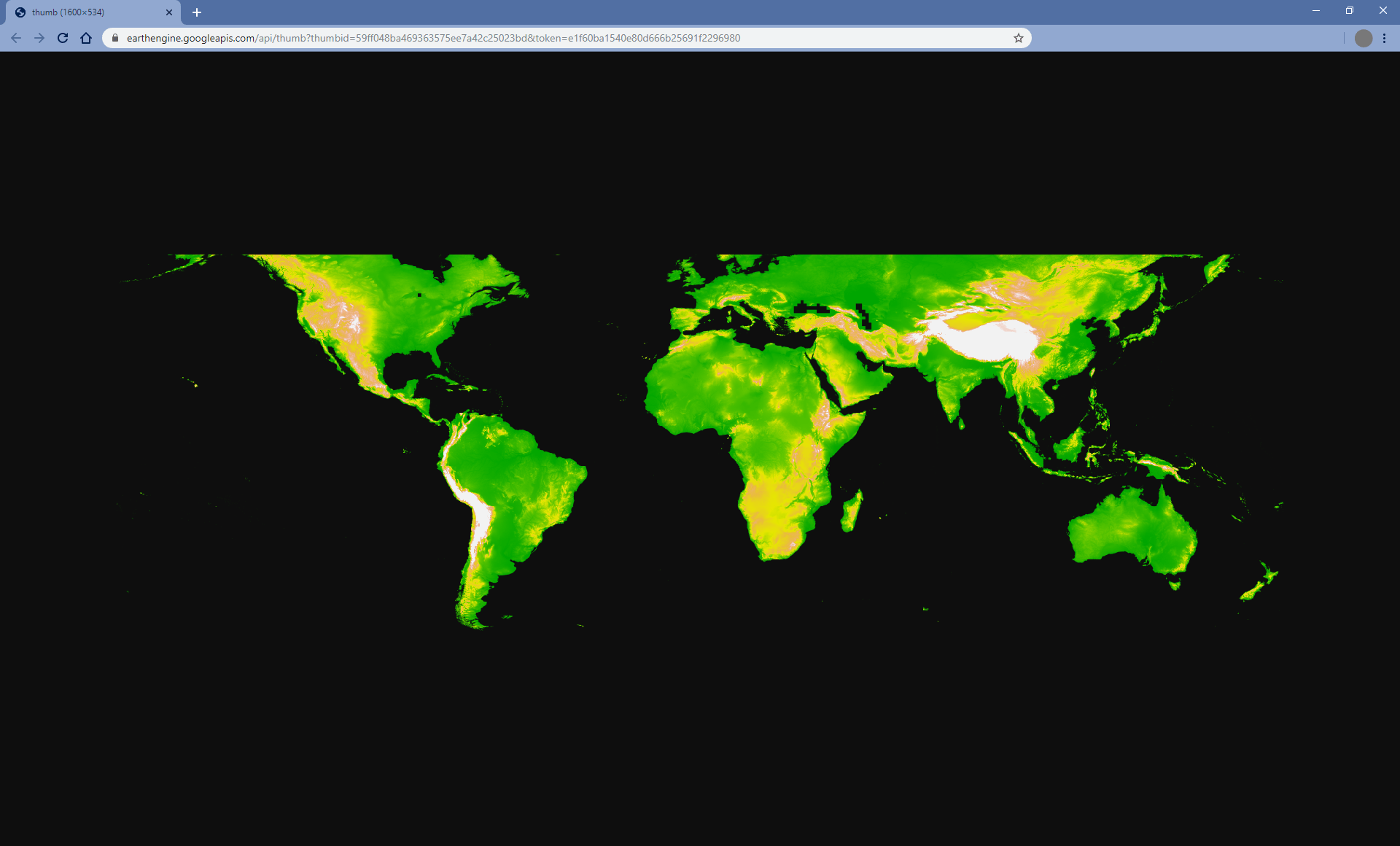
다음은 getThumbURL() 매개변수 인수의 다양한 조합을 보여주는 일련의 예입니다. 이 스크립트를 실행할 때 출력된 URL을 클릭하여 썸네일을 봅니다.
코드 편집기 (JavaScript)
// Fetch a digital elevation model.
var image = ee.Image('CGIAR/SRTM90_V4');

// Request a default thumbnail of the DEM with defined linear stretch.
// Set masked pixels (ocean) to 1000 so they map as gray.
var thumbnail1 = image.unmask(1000).getThumbURL({
  'min': 0,
  'max': 3000,
  'dimensions': 500,
});
print('Default extent:', thumbnail1);

// Specify region by rectangle, define palette, set larger aspect dimension size.
var thumbnail2 = image.getThumbURL({
  'min': 0,
  'max': 3000,
  'palette': ['00A600','63C600','E6E600','E9BD3A','ECB176','EFC2B3','F2F2F2'],
  'dimensions': 500,
  'region': ee.Geometry.Rectangle([-84.6, -55.9, -32.9, 15.7]),
});
print('Rectangle region and palette:', thumbnail2);

// Specify region by a linear ring and set display CRS as Web Mercator.
var thumbnail3 = image.getThumbURL({
  'min': 0,
  'max': 3000,
  'palette': ['00A600','63C600','E6E600','E9BD3A','ECB176','EFC2B3','F2F2F2'],
  'region': ee.Geometry.LinearRing([[-84.6, 15.7], [-84.6, -55.9], [-32.9, -55.9]]),
  'dimensions': 500,
  'crs': 'EPSG:3857'
});
print('Linear ring region and specified crs', thumbnail3);
import ee
import geemap.core as geemap
Colab (Python)
# Fetch a digital elevation model.
image = ee.Image('CGIAR/SRTM90_V4')

# Request a default thumbnail of the DEM with defined linear stretch.
# Set masked pixels (ocean) to 1000 so they map as gray.
thumbnail_1 = image.unmask(1000).getThumbURL({
    'min': 0,
    'max': 3000,
    'dimensions': 500,
})
print('Default extent:', thumbnail_1)

# Specify region by rectangle, define palette, set larger aspect dimension size.
thumbnail_2 = image.getThumbURL({
    'min': 0,
    'max': 3000,
    'palette': [
        '00A600',
        '63C600',
        'E6E600',
        'E9BD3A',
        'ECB176',
        'EFC2B3',
        'F2F2F2',
    ],
    'dimensions': 500,
    'region': ee.Geometry.Rectangle([-84.6, -55.9, -32.9, 15.7]),
})
print('Rectangle region and palette:', thumbnail_2)

# Specify region by a linear ring and set display CRS as Web Mercator.
thumbnail_3 = image.getThumbURL({
    'min': 0,
    'max': 3000,
    'palette': [
        '00A600',
        '63C600',
        'E6E600',
        'E9BD3A',
        'ECB176',
        'EFC2B3',
        'F2F2F2',
    ],
    'region': ee.Geometry.LinearRing(
        [[-84.6, 15.7], [-84.6, -55.9], [-32.9, -55.9]]
    ),
    'dimensions': 500,
    'crs': 'EPSG:3857',
})
print('Linear ring region and specified crs:', thumbnail_3)