Trasformazioni spettrali

Esegui in Google Colab

Visualizza il codice sorgente su GitHub

In Earth Engine esistono diversi metodi di trasformazione spettrale. Sono inclusi metodi di istanza su immagini come normalizedDifference(), unmix(), rgbToHsv() e hsvToRgb().

Affilatura della panoramica

L'aumento della nitidezza migliora la risoluzione di un'immagine multibanda tramite il miglioramento fornito da un'immagine pancromatica corrispondente con una risoluzione più fine. I metodi rgbToHsv() e hsvToRgb() sono utili per la sfocatura panoramica.

Editor di codice (JavaScript)

// Load a Landsat 8 top-of-atmosphere reflectance image.
var image = ee.Image('LANDSAT/LC08/C02/T1_TOA/LC08_044034_20140318');
Map.addLayer(
    image,
    {bands: ['B4', 'B3', 'B2'], min: 0, max: 0.25, gamma: [1.1, 1.1, 1]},
    'rgb');

// Convert the RGB bands to the HSV color space.
var hsv = image.select(['B4', 'B3', 'B2']).rgbToHsv();

// Swap in the panchromatic band and convert back to RGB.
var sharpened = ee.Image.cat([
  hsv.select('hue'), hsv.select('saturation'), image.select('B8')
]).hsvToRgb();

// Display the pan-sharpened result.
Map.setCenter(-122.44829, 37.76664, 13);
Map.addLayer(sharpened,
             {min: 0, max: 0.25, gamma: [1.3, 1.3, 1.3]},
             'pan-sharpened');

Configurazione di Python

Per informazioni sull'API Python e sull'utilizzo di geemap per lo sviluppo interattivo, consulta la pagina Ambiente Python.

import ee
import geemap.core as geemap

Colab (Python)

# Load a Landsat 8 top-of-atmosphere reflectance image.
image = ee.Image('LANDSAT/LC08/C02/T1_TOA/LC08_044034_20140318')

# Convert the RGB bands to the HSV color space.
hsv = image.select(['B4', 'B3', 'B2']).rgbToHsv()

# Swap in the panchromatic band and convert back to RGB.
sharpened = ee.Image.cat(
    [hsv.select('hue'), hsv.select('saturation'), image.select('B8')]
).hsvToRgb()

# Define a map centered on San Francisco, California.
map_sharpened = geemap.Map(center=[37.76664, -122.44829], zoom=13)

# Add the image layers to the map and display it.
map_sharpened.add_layer(
    image,
    {
        'bands': ['B4', 'B3', 'B2'],
        'min': 0,
        'max': 0.25,
        'gamma': [1.1, 1.1, 1],
    },
    'rgb',
)
map_sharpened.add_layer(
    sharpened,
    {'min': 0, 'max': 0.25, 'gamma': [1.3, 1.3, 1.3]},
    'pan-sharpened',
)
display(map_sharpened)

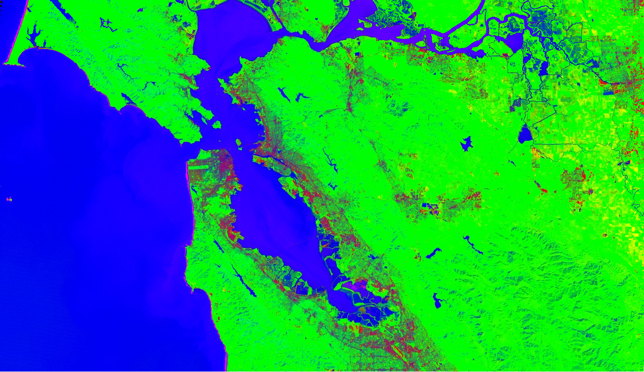
Scomposizione spettrale

L'analisi spettrale è implementata in Earth Engine come metodo image.unmix(). Per metodi più flessibili, consulta la pagina Trasformazioni di array. Di seguito è riportato un esempio di scomposizione di Landsat 5 con componenti finali predeterminati di vegetazione, acqua e aree urbane:

Editor di codice (JavaScript)

// Load a Landsat 5 image and select the bands we want to unmix.
var bands = ['B1', 'B2', 'B3', 'B4', 'B5', 'B6', 'B7'];
var image = ee.Image('LANDSAT/LT05/C02/T1/LT05_044034_20080214')
  .select(bands);
Map.setCenter(-122.1899, 37.5010, 10); // San Francisco Bay
Map.addLayer(image, {bands: ['B4', 'B3', 'B2'], min: 0, max: 128}, 'image');

// Define spectral endmembers.
var urban = [88, 42, 48, 38, 86, 115, 59];
var veg = [50, 21, 20, 35, 50, 110, 23];
var water = [51, 20, 14, 9, 7, 116, 4];

// Unmix the image.
var fractions = image.unmix([urban, veg, water]);
Map.addLayer(fractions, {}, 'unmixed');

Configurazione di Python

Per informazioni sull'API Python e sull'utilizzo di geemap per lo sviluppo interattivo, consulta la pagina Ambiente Python.

import ee
import geemap.core as geemap

Colab (Python)

# Load a Landsat 5 image and select the bands we want to unmix.
bands = ['B1', 'B2', 'B3', 'B4', 'B5', 'B6', 'B7']
image = ee.Image('LANDSAT/LT05/C02/T1/LT05_044034_20080214').select(bands)

# Define spectral endmembers.
urban = [88, 42, 48, 38, 86, 115, 59]
veg = [50, 21, 20, 35, 50, 110, 23]
water = [51, 20, 14, 9, 7, 116, 4]

# Unmix the image.
fractions = image.unmix([urban, veg, water])

# Define a map centered on San Francisco Bay.
map_fractions = geemap.Map(center=[37.5010, -122.1899], zoom=10)

# Add the image layers to the map and display it.
map_fractions.add_layer(
    image, {'bands': ['B4', 'B3', 'B2'], 'min': 0, 'max': 128}, 'image'
)
map_fractions.add_layer(fractions, None, 'unmixed')
display(map_fractions)

Figura 1. Immagini Landsat 5 non mescolate in frazioni urbane (rosse), vegetazione (verdi) e acqua (blu). Baia di San Francisco, California, Stati Uniti.