Solving an LP Problem

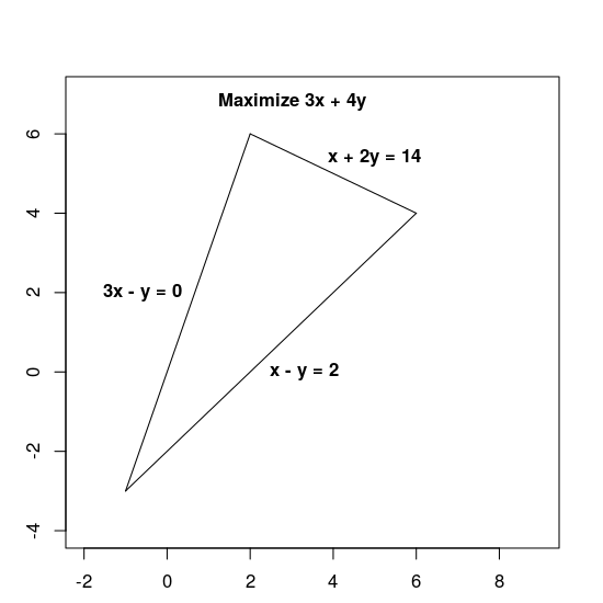
The following sections present an example of an LP problem and show how to solve it. Here's the problem:

Maximize 3x + 4y subject to the following constraints:

x + 2y ≤ 14
3x - y ≥ 0
x - y ≤ 2

Both the objective function, 3x + 4y, and the constraints are given by linear expressions, which makes this a linear problem.

The constraints define the feasible region, which is the triangle shown below, including its interior.

Basic steps for solving an LP problem

To solve a LP problem, your program should include the following steps:

Import the linear solver wrapper,
declare the LP solver,
define the variables,
define the constraints,
define the objective,
call the LP solver; and
display the solution

Solution using the MPSolver

The following section present a program that solves the problem using the MPSolver wrapper and an LP solver.

Note. To run the program below, you need to install OR-Tools.

The primary OR-Tools linear optimization solver is Glop, Google's in-house linear programming solver. It's fast, memory efficient, and numerically stable.

Import the linear solver wrapper

Import (or include) the OR-Tools linear solver wrapper, an interface for MIP solvers and linear solvers, as shown below.

Python

from ortools.linear_solver import pywraplp

C++

#include <iostream>
#include <memory>

#include "ortools/linear_solver/linear_solver.h"

Java

import com.google.ortools.Loader;
import com.google.ortools.linearsolver.MPConstraint;
import com.google.ortools.linearsolver.MPObjective;
import com.google.ortools.linearsolver.MPSolver;
import com.google.ortools.linearsolver.MPVariable;

C#

using System;
using Google.OrTools.LinearSolver;

Declare the LP solver

MPsolver is a wrapper for several different solvers, including Glop. The code below declares the GLOP solver.

Python

solver = pywraplp.Solver.CreateSolver("GLOP")
if not solver:
    return

C++

std::unique_ptr<MPSolver> solver(MPSolver::CreateSolver("SCIP"));
if (!solver) {
  LOG(WARNING) << "SCIP solver unavailable.";
  return;
}

Java

MPSolver solver = MPSolver.createSolver("GLOP");

C#

Solver solver = Solver.CreateSolver("GLOP");
if (solver is null)
{
    return;
}

Note: Substitute PDLP for GLOP to use an alternative LP solver. For more details on choosing solvers, see advanced LP solving, and for installation of third-party solvers, see the installation guide.

Create the variables

First, create variables x and y whose values are in the range from 0 to infinity.

Python

x = solver.NumVar(0, solver.infinity(), "x")
y = solver.NumVar(0, solver.infinity(), "y")

print("Number of variables =", solver.NumVariables())

C++

const double infinity = solver->infinity();
// x and y are non-negative variables.
MPVariable* const x = solver->MakeNumVar(0.0, infinity, "x");
MPVariable* const y = solver->MakeNumVar(0.0, infinity, "y");
LOG(INFO) << "Number of variables = " << solver->NumVariables();

Java

double infinity = java.lang.Double.POSITIVE_INFINITY;
// x and y are continuous non-negative variables.
MPVariable x = solver.makeNumVar(0.0, infinity, "x");
MPVariable y = solver.makeNumVar(0.0, infinity, "y");
System.out.println("Number of variables = " + solver.numVariables());

C#

Variable x = solver.MakeNumVar(0.0, double.PositiveInfinity, "x");
Variable y = solver.MakeNumVar(0.0, double.PositiveInfinity, "y");

Console.WriteLine("Number of variables = " + solver.NumVariables());

Define the constraints

Next, define the constraints on the variables. Give each constraint a unique name (such as constraint0), and then define the coefficients for the constraint.

Python

# Constraint 0: x + 2y <= 14.
solver.Add(x + 2 * y <= 14.0)

# Constraint 1: 3x - y >= 0.
solver.Add(3 * x - y >= 0.0)

# Constraint 2: x - y <= 2.
solver.Add(x - y <= 2.0)

print("Number of constraints =", solver.NumConstraints())

C++

// x + 2*y <= 14.
MPConstraint* const c0 = solver->MakeRowConstraint(-infinity, 14.0);
c0->SetCoefficient(x, 1);
c0->SetCoefficient(y, 2);

// 3*x - y >= 0.
MPConstraint* const c1 = solver->MakeRowConstraint(0.0, infinity);
c1->SetCoefficient(x, 3);
c1->SetCoefficient(y, -1);

// x - y <= 2.
MPConstraint* const c2 = solver->MakeRowConstraint(-infinity, 2.0);
c2->SetCoefficient(x, 1);
c2->SetCoefficient(y, -1);
LOG(INFO) << "Number of constraints = " << solver->NumConstraints();

Java

// x + 2*y <= 14.
MPConstraint c0 = solver.makeConstraint(-infinity, 14.0, "c0");
c0.setCoefficient(x, 1);
c0.setCoefficient(y, 2);

// 3*x - y >= 0.
MPConstraint c1 = solver.makeConstraint(0.0, infinity, "c1");
c1.setCoefficient(x, 3);
c1.setCoefficient(y, -1);

// x - y <= 2.
MPConstraint c2 = solver.makeConstraint(-infinity, 2.0, "c2");
c2.setCoefficient(x, 1);
c2.setCoefficient(y, -1);
System.out.println("Number of constraints = " + solver.numConstraints());

C#

// x + 2y <= 14.
solver.Add(x + 2 * y <= 14.0);

// 3x - y >= 0.
solver.Add(3 * x - y >= 0.0);

// x - y <= 2.
solver.Add(x - y <= 2.0);

Console.WriteLine("Number of constraints = " + solver.NumConstraints());

Define the objective function

The following code defines the objective function, 3x + 4y, and specifies that this is a maximization problem.

Python

# Objective function: 3x + 4y.
solver.Maximize(3 * x + 4 * y)

C++

// Objective function: 3x + 4y.
MPObjective* const objective = solver->MutableObjective();
objective->SetCoefficient(x, 3);
objective->SetCoefficient(y, 4);
objective->SetMaximization();

Java

// Maximize 3 * x + 4 * y.
MPObjective objective = solver.objective();
objective.setCoefficient(x, 3);
objective.setCoefficient(y, 4);
objective.setMaximization();

C#

// Objective function: 3x + 4y.
solver.Maximize(3 * x + 4 * y);

Invoke the solver

The following code invokes the solver.

Python

print(f"Solving with {solver.SolverVersion()}")
status = solver.Solve()

C++

const MPSolver::ResultStatus result_status = solver->Solve();
// Check that the problem has an optimal solution.
if (result_status != MPSolver::OPTIMAL) {
  LOG(FATAL) << "The problem does not have an optimal solution!";
}

Java

final MPSolver.ResultStatus resultStatus = solver.solve();

C#

Solver.ResultStatus resultStatus = solver.Solve();

Display the solution

The following code displays the solution.

Python

if status == pywraplp.Solver.OPTIMAL:
    print("Solution:")
    print(f"Objective value = {solver.Objective().Value():0.1f}")
    print(f"x = {x.solution_value():0.1f}")
    print(f"y = {y.solution_value():0.1f}")
else:
    print("The problem does not have an optimal solution.")

C++

LOG(INFO) << "Solution:";
LOG(INFO) << "Optimal objective value = " << objective->Value();
LOG(INFO) << x->name() << " = " << x->solution_value();
LOG(INFO) << y->name() << " = " << y->solution_value();

Java

if (resultStatus == MPSolver.ResultStatus.OPTIMAL) {
  System.out.println("Solution:");
  System.out.println("Objective value = " + objective.value());
  System.out.println("x = " + x.solutionValue());
  System.out.println("y = " + y.solutionValue());
} else {
  System.err.println("The problem does not have an optimal solution!");
}

C#

// Check that the problem has an optimal solution.
if (resultStatus != Solver.ResultStatus.OPTIMAL)
{
    Console.WriteLine("The problem does not have an optimal solution!");
    return;
}
Console.WriteLine("Solution:");
Console.WriteLine("Objective value = " + solver.Objective().Value());
Console.WriteLine("x = " + x.SolutionValue());
Console.WriteLine("y = " + y.SolutionValue());

The complete programs

The complete programs are shown below.

Python

from ortools.linear_solver import pywraplp


def LinearProgrammingExample():
    """Linear programming sample."""
    # Instantiate a Glop solver, naming it LinearExample.
    solver = pywraplp.Solver.CreateSolver("GLOP")
    if not solver:
        return

    # Create the two variables and let them take on any non-negative value.
    x = solver.NumVar(0, solver.infinity(), "x")
    y = solver.NumVar(0, solver.infinity(), "y")

    print("Number of variables =", solver.NumVariables())

    # Constraint 0: x + 2y <= 14.
    solver.Add(x + 2 * y <= 14.0)

    # Constraint 1: 3x - y >= 0.
    solver.Add(3 * x - y >= 0.0)

    # Constraint 2: x - y <= 2.
    solver.Add(x - y <= 2.0)

    print("Number of constraints =", solver.NumConstraints())

    # Objective function: 3x + 4y.
    solver.Maximize(3 * x + 4 * y)

    # Solve the system.
    print(f"Solving with {solver.SolverVersion()}")
    status = solver.Solve()

    if status == pywraplp.Solver.OPTIMAL:
        print("Solution:")
        print(f"Objective value = {solver.Objective().Value():0.1f}")
        print(f"x = {x.solution_value():0.1f}")
        print(f"y = {y.solution_value():0.1f}")
    else:
        print("The problem does not have an optimal solution.")

    print("\nAdvanced usage:")
    print(f"Problem solved in {solver.wall_time():d} milliseconds")
    print(f"Problem solved in {solver.iterations():d} iterations")


LinearProgrammingExample()

C++

#include <iostream>
#include <memory>

#include "ortools/linear_solver/linear_solver.h"

namespace operations_research {
void LinearProgrammingExample() {
  std::unique_ptr<MPSolver> solver(MPSolver::CreateSolver("SCIP"));
  if (!solver) {
    LOG(WARNING) << "SCIP solver unavailable.";
    return;
  }

  const double infinity = solver->infinity();
  // x and y are non-negative variables.
  MPVariable* const x = solver->MakeNumVar(0.0, infinity, "x");
  MPVariable* const y = solver->MakeNumVar(0.0, infinity, "y");
  LOG(INFO) << "Number of variables = " << solver->NumVariables();

  // x + 2*y <= 14.
  MPConstraint* const c0 = solver->MakeRowConstraint(-infinity, 14.0);
  c0->SetCoefficient(x, 1);
  c0->SetCoefficient(y, 2);

  // 3*x - y >= 0.
  MPConstraint* const c1 = solver->MakeRowConstraint(0.0, infinity);
  c1->SetCoefficient(x, 3);
  c1->SetCoefficient(y, -1);

  // x - y <= 2.
  MPConstraint* const c2 = solver->MakeRowConstraint(-infinity, 2.0);
  c2->SetCoefficient(x, 1);
  c2->SetCoefficient(y, -1);
  LOG(INFO) << "Number of constraints = " << solver->NumConstraints();

  // Objective function: 3x + 4y.
  MPObjective* const objective = solver->MutableObjective();
  objective->SetCoefficient(x, 3);
  objective->SetCoefficient(y, 4);
  objective->SetMaximization();

  const MPSolver::ResultStatus result_status = solver->Solve();
  // Check that the problem has an optimal solution.
  if (result_status != MPSolver::OPTIMAL) {
    LOG(FATAL) << "The problem does not have an optimal solution!";
  }

  LOG(INFO) << "Solution:";
  LOG(INFO) << "Optimal objective value = " << objective->Value();
  LOG(INFO) << x->name() << " = " << x->solution_value();
  LOG(INFO) << y->name() << " = " << y->solution_value();
}
}  // namespace operations_research

int main(int argc, char** argv) {
  operations_research::LinearProgrammingExample();
  return EXIT_SUCCESS;
}

Java

package com.google.ortools.linearsolver.samples;
import com.google.ortools.Loader;
import com.google.ortools.linearsolver.MPConstraint;
import com.google.ortools.linearsolver.MPObjective;
import com.google.ortools.linearsolver.MPSolver;
import com.google.ortools.linearsolver.MPVariable;

/** Simple linear programming example. */
public final class LinearProgrammingExample {
  public static void main(String[] args) {
    Loader.loadNativeLibraries();
    MPSolver solver = MPSolver.createSolver("GLOP");

    double infinity = java.lang.Double.POSITIVE_INFINITY;
    // x and y are continuous non-negative variables.
    MPVariable x = solver.makeNumVar(0.0, infinity, "x");
    MPVariable y = solver.makeNumVar(0.0, infinity, "y");
    System.out.println("Number of variables = " + solver.numVariables());

    // x + 2*y <= 14.
    MPConstraint c0 = solver.makeConstraint(-infinity, 14.0, "c0");
    c0.setCoefficient(x, 1);
    c0.setCoefficient(y, 2);

    // 3*x - y >= 0.
    MPConstraint c1 = solver.makeConstraint(0.0, infinity, "c1");
    c1.setCoefficient(x, 3);
    c1.setCoefficient(y, -1);

    // x - y <= 2.
    MPConstraint c2 = solver.makeConstraint(-infinity, 2.0, "c2");
    c2.setCoefficient(x, 1);
    c2.setCoefficient(y, -1);
    System.out.println("Number of constraints = " + solver.numConstraints());

    // Maximize 3 * x + 4 * y.
    MPObjective objective = solver.objective();
    objective.setCoefficient(x, 3);
    objective.setCoefficient(y, 4);
    objective.setMaximization();

    final MPSolver.ResultStatus resultStatus = solver.solve();

    if (resultStatus == MPSolver.ResultStatus.OPTIMAL) {
      System.out.println("Solution:");
      System.out.println("Objective value = " + objective.value());
      System.out.println("x = " + x.solutionValue());
      System.out.println("y = " + y.solutionValue());
    } else {
      System.err.println("The problem does not have an optimal solution!");
    }

    System.out.println("\nAdvanced usage:");
    System.out.println("Problem solved in " + solver.wallTime() + " milliseconds");
    System.out.println("Problem solved in " + solver.iterations() + " iterations");
  }

  private LinearProgrammingExample() {}
}

C#

using System;
using Google.OrTools.LinearSolver;

public class LinearProgrammingExample
{
    static void Main()
    {
        Solver solver = Solver.CreateSolver("GLOP");
        if (solver is null)
        {
            return;
        }
        // x and y are continuous non-negative variables.
        Variable x = solver.MakeNumVar(0.0, double.PositiveInfinity, "x");
        Variable y = solver.MakeNumVar(0.0, double.PositiveInfinity, "y");

        Console.WriteLine("Number of variables = " + solver.NumVariables());

        // x + 2y <= 14.
        solver.Add(x + 2 * y <= 14.0);

        // 3x - y >= 0.
        solver.Add(3 * x - y >= 0.0);

        // x - y <= 2.
        solver.Add(x - y <= 2.0);

        Console.WriteLine("Number of constraints = " + solver.NumConstraints());

        // Objective function: 3x + 4y.
        solver.Maximize(3 * x + 4 * y);

        Solver.ResultStatus resultStatus = solver.Solve();

        // Check that the problem has an optimal solution.
        if (resultStatus != Solver.ResultStatus.OPTIMAL)
        {
            Console.WriteLine("The problem does not have an optimal solution!");
            return;
        }
        Console.WriteLine("Solution:");
        Console.WriteLine("Objective value = " + solver.Objective().Value());
        Console.WriteLine("x = " + x.SolutionValue());
        Console.WriteLine("y = " + y.SolutionValue());

        Console.WriteLine("\nAdvanced usage:");
        Console.WriteLine("Problem solved in " + solver.WallTime() + " milliseconds");
        Console.WriteLine("Problem solved in " + solver.Iterations() + " iterations");
    }
}

Optimal solution

The program returns the optimal solution to the problem, as shown below.

Number of variables = 2
Number of constraints = 3
Solution:
x = 6.0
y = 4.0
Optimal objective value = 34.0

Here is a graph showing the solution:

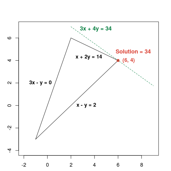
The dashed green line is defined by setting the objective function equal to its optimal value of 34. Any line whose equation has the form 3x + 4y = c is parallel to the dashed line, and 34 is the largest value of c for which the line intersects the feasible region.

To learn more about solving linear optimization problems, see advanced LP solving.