Solving a MIP Problem

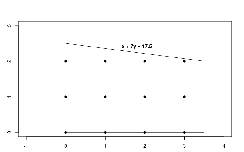
The following sections present an example of a MIP problem and show how to solve it. Here's the problem:

Maximize x + 10y subject to the following constraints:

1. x + 7y ≤ 17.5
2. 0 ≤ x ≤ 3.5
3. 0 ≤ y
4. x, y integers

Since the constraints are linear, this is just a linear optimization problem in which the solutions are required to be integers. The graph below shows the integer points in the feasible region for the problem.

Notice that this problem is very similar to the linear optimization problem described in Solving an LP Problem, but in this case we require the solutions to be integers.

Basic steps for solving a MIP problem

To solve a MIP problem, your program should include the following steps:

1. Import the linear solver wrapper,
2. declare the MIP solver,
3. define the variables,
4. define the constraints,
5. define the objective,
6. call the MIP solver and
7. display the solution

Solution using the MPSolver

The following section present a program that solves the problem using the MPSolver wrapper and a MIP solver.

Note: To run the program below, you need to install OR-Tools.

The default OR-Tools MIP solver is SCIP.

Import the linear solver wrapper

Import (or include) the OR-Tools linear solver wrapper, an interface for MIP solvers and linear solvers, as shown below.

Python

from ortools.linear_solver import pywraplp

C++

#include <memory>

#include "ortools/linear_solver/linear_solver.h"

Java

import com.google.ortools.Loader;
import com.google.ortools.linearsolver.MPConstraint;
import com.google.ortools.linearsolver.MPObjective;
import com.google.ortools.linearsolver.MPSolver;
import com.google.ortools.linearsolver.MPVariable;

C#

using System;
using Google.OrTools.LinearSolver;

Declare the MIP solver

The following code declares the MIP solver for the problem. This example uses the third-party solver SCIP.

Note: If you build OR-Tools from source and wish to install and use a different solver, see the installation guide guide for your platform.

Python

# Create the mip solver with the SCIP backend.
solver = pywraplp.Solver.CreateSolver("SAT")
if not solver:
    return

C++

// Create the mip solver with the SCIP backend.
std::unique_ptr<MPSolver> solver(MPSolver::CreateSolver("SCIP"));
if (!solver) {
  LOG(WARNING) << "SCIP solver unavailable.";
  return;
}

Java

// Create the linear solver with the SCIP backend.
MPSolver solver = MPSolver.createSolver("SCIP");
if (solver == null) {
  System.out.println("Could not create solver SCIP");
  return;
}

C#

// Create the linear solver with the SCIP backend.
Solver solver = Solver.CreateSolver("SCIP");
if (solver is null)
{
    return;
}

Define the variables

The following code defines the variables in the problem.

Python

infinity = solver.infinity()
# x and y are integer non-negative variables.
x = solver.IntVar(0.0, infinity, "x")
y = solver.IntVar(0.0, infinity, "y")

print("Number of variables =", solver.NumVariables())

C++

const double infinity = solver->infinity();
// x and y are integer non-negative variables.
MPVariable* const x = solver->MakeIntVar(0.0, infinity, "x");
MPVariable* const y = solver->MakeIntVar(0.0, infinity, "y");

LOG(INFO) << "Number of variables = " << solver->NumVariables();

Java

double infinity = java.lang.Double.POSITIVE_INFINITY;
// x and y are integer non-negative variables.
MPVariable x = solver.makeIntVar(0.0, infinity, "x");
MPVariable y = solver.makeIntVar(0.0, infinity, "y");

System.out.println("Number of variables = " + solver.numVariables());

C#

// x and y are integer non-negative variables.
Variable x = solver.MakeIntVar(0.0, double.PositiveInfinity, "x");
Variable y = solver.MakeIntVar(0.0, double.PositiveInfinity, "y");

Console.WriteLine("Number of variables = " + solver.NumVariables());

The program uses the MakeIntVar method (or a variant, depending on the coding language) to create variables x and y that take on non-negative integer values.

Define the constraints

The following code defines the constraints for the problem.

Python

# x + 7 * y <= 17.5.
solver.Add(x + 7 * y <= 17.5)

# x <= 3.5.
solver.Add(x <= 3.5)

print("Number of constraints =", solver.NumConstraints())

C++

// x + 7 * y <= 17.5.
MPConstraint* const c0 = solver->MakeRowConstraint(-infinity, 17.5, "c0");
c0->SetCoefficient(x, 1);
c0->SetCoefficient(y, 7);

// x <= 3.5.
MPConstraint* const c1 = solver->MakeRowConstraint(-infinity, 3.5, "c1");
c1->SetCoefficient(x, 1);
c1->SetCoefficient(y, 0);

LOG(INFO) << "Number of constraints = " << solver->NumConstraints();

Java

// x + 7 * y <= 17.5.
MPConstraint c0 = solver.makeConstraint(-infinity, 17.5, "c0");
c0.setCoefficient(x, 1);
c0.setCoefficient(y, 7);

// x <= 3.5.
MPConstraint c1 = solver.makeConstraint(-infinity, 3.5, "c1");
c1.setCoefficient(x, 1);
c1.setCoefficient(y, 0);

System.out.println("Number of constraints = " + solver.numConstraints());

C#

// x + 7 * y <= 17.5.
solver.Add(x + 7 * y <= 17.5);

// x <= 3.5.
solver.Add(x <= 3.5);

Console.WriteLine("Number of constraints = " + solver.NumConstraints());

Define the objective

The following code defines the objective function for the problem.

Python

# Maximize x + 10 * y.
solver.Maximize(x + 10 * y)

C++

// Maximize x + 10 * y.
MPObjective* const objective = solver->MutableObjective();
objective->SetCoefficient(x, 1);
objective->SetCoefficient(y, 10);
objective->SetMaximization();

Java

// Maximize x + 10 * y.
MPObjective objective = solver.objective();
objective.setCoefficient(x, 1);
objective.setCoefficient(y, 10);
objective.setMaximization();

C#

// Maximize x + 10 * y.
solver.Maximize(x + 10 * y);

Call the solver

The following code calls the solver.

Python

print(f"Solving with {solver.SolverVersion()}")
status = solver.Solve()

C++

const MPSolver::ResultStatus result_status = solver->Solve();
// Check that the problem has an optimal solution.
if (result_status != MPSolver::OPTIMAL) {
  LOG(FATAL) << "The problem does not have an optimal solution!";
}

Java

final MPSolver.ResultStatus resultStatus = solver.solve();

C#

Solver.ResultStatus resultStatus = solver.Solve();

Display the solution

The following code displays the solution.

Python

if status == pywraplp.Solver.OPTIMAL:
    print("Solution:")
    print("Objective value =", solver.Objective().Value())
    print("x =", x.solution_value())
    print("y =", y.solution_value())
else:
    print("The problem does not have an optimal solution.")

C++

LOG(INFO) << "Solution:";
LOG(INFO) << "Objective value = " << objective->Value();
LOG(INFO) << "x = " << x->solution_value();
LOG(INFO) << "y = " << y->solution_value();

Java

if (resultStatus == MPSolver.ResultStatus.OPTIMAL) {
  System.out.println("Solution:");
  System.out.println("Objective value = " + objective.value());
  System.out.println("x = " + x.solutionValue());
  System.out.println("y = " + y.solutionValue());
} else {
  System.err.println("The problem does not have an optimal solution!");
}

C#

// Check that the problem has an optimal solution.
if (resultStatus != Solver.ResultStatus.OPTIMAL)
{
    Console.WriteLine("The problem does not have an optimal solution!");
    return;
}
Console.WriteLine("Solution:");
Console.WriteLine("Objective value = " + solver.Objective().Value());
Console.WriteLine("x = " + x.SolutionValue());
Console.WriteLine("y = " + y.SolutionValue());

Here is the solution to the problem.

Number of variables = 2
Number of constraints = 2
Solution:
Objective value = 23
x = 3
y = 2

The optimal value of the objective function is 23, which occurs at the point x = 3, y = 2.

Complete programs

Here are the complete programs.

Python

from ortools.linear_solver import pywraplp


def main():
    # Create the mip solver with the SCIP backend.
    solver = pywraplp.Solver.CreateSolver("SAT")
    if not solver:
        return

    infinity = solver.infinity()
    # x and y are integer non-negative variables.
    x = solver.IntVar(0.0, infinity, "x")
    y = solver.IntVar(0.0, infinity, "y")

    print("Number of variables =", solver.NumVariables())

    # x + 7 * y <= 17.5.
    solver.Add(x + 7 * y <= 17.5)

    # x <= 3.5.
    solver.Add(x <= 3.5)

    print("Number of constraints =", solver.NumConstraints())

    # Maximize x + 10 * y.
    solver.Maximize(x + 10 * y)

    print(f"Solving with {solver.SolverVersion()}")
    status = solver.Solve()

    if status == pywraplp.Solver.OPTIMAL:
        print("Solution:")
        print("Objective value =", solver.Objective().Value())
        print("x =", x.solution_value())
        print("y =", y.solution_value())
    else:
        print("The problem does not have an optimal solution.")

    print("\nAdvanced usage:")
    print(f"Problem solved in {solver.wall_time():d} milliseconds")
    print(f"Problem solved in {solver.iterations():d} iterations")
    print(f"Problem solved in {solver.nodes():d} branch-and-bound nodes")


if __name__ == "__main__":
    main()

C++

#include <memory>

#include "ortools/linear_solver/linear_solver.h"

namespace operations_research {
void SimpleMipProgram() {
  // Create the mip solver with the SCIP backend.
  std::unique_ptr<MPSolver> solver(MPSolver::CreateSolver("SCIP"));
  if (!solver) {
    LOG(WARNING) << "SCIP solver unavailable.";
    return;
  }

  const double infinity = solver->infinity();
  // x and y are integer non-negative variables.
  MPVariable* const x = solver->MakeIntVar(0.0, infinity, "x");
  MPVariable* const y = solver->MakeIntVar(0.0, infinity, "y");

  LOG(INFO) << "Number of variables = " << solver->NumVariables();

  // x + 7 * y <= 17.5.
  MPConstraint* const c0 = solver->MakeRowConstraint(-infinity, 17.5, "c0");
  c0->SetCoefficient(x, 1);
  c0->SetCoefficient(y, 7);

  // x <= 3.5.
  MPConstraint* const c1 = solver->MakeRowConstraint(-infinity, 3.5, "c1");
  c1->SetCoefficient(x, 1);
  c1->SetCoefficient(y, 0);

  LOG(INFO) << "Number of constraints = " << solver->NumConstraints();

  // Maximize x + 10 * y.
  MPObjective* const objective = solver->MutableObjective();
  objective->SetCoefficient(x, 1);
  objective->SetCoefficient(y, 10);
  objective->SetMaximization();

  const MPSolver::ResultStatus result_status = solver->Solve();
  // Check that the problem has an optimal solution.
  if (result_status != MPSolver::OPTIMAL) {
    LOG(FATAL) << "The problem does not have an optimal solution!";
  }

  LOG(INFO) << "Solution:";
  LOG(INFO) << "Objective value = " << objective->Value();
  LOG(INFO) << "x = " << x->solution_value();
  LOG(INFO) << "y = " << y->solution_value();

  LOG(INFO) << "\nAdvanced usage:";
  LOG(INFO) << "Problem solved in " << solver->wall_time() << " milliseconds";
  LOG(INFO) << "Problem solved in " << solver->iterations() << " iterations";
  LOG(INFO) << "Problem solved in " << solver->nodes()
            << " branch-and-bound nodes";
}
}  // namespace operations_research

int main(int argc, char** argv) {
  operations_research::SimpleMipProgram();
  return EXIT_SUCCESS;
}

Java

package com.google.ortools.linearsolver.samples;
import com.google.ortools.Loader;
import com.google.ortools.linearsolver.MPConstraint;
import com.google.ortools.linearsolver.MPObjective;
import com.google.ortools.linearsolver.MPSolver;
import com.google.ortools.linearsolver.MPVariable;

/** Minimal Mixed Integer Programming example to showcase calling the solver. */
public final class SimpleMipProgram {
  public static void main(String[] args) {
    Loader.loadNativeLibraries();
    // Create the linear solver with the SCIP backend.
    MPSolver solver = MPSolver.createSolver("SCIP");
    if (solver == null) {
      System.out.println("Could not create solver SCIP");
      return;
    }

    double infinity = java.lang.Double.POSITIVE_INFINITY;
    // x and y are integer non-negative variables.
    MPVariable x = solver.makeIntVar(0.0, infinity, "x");
    MPVariable y = solver.makeIntVar(0.0, infinity, "y");

    System.out.println("Number of variables = " + solver.numVariables());

    // x + 7 * y <= 17.5.
    MPConstraint c0 = solver.makeConstraint(-infinity, 17.5, "c0");
    c0.setCoefficient(x, 1);
    c0.setCoefficient(y, 7);

    // x <= 3.5.
    MPConstraint c1 = solver.makeConstraint(-infinity, 3.5, "c1");
    c1.setCoefficient(x, 1);
    c1.setCoefficient(y, 0);

    System.out.println("Number of constraints = " + solver.numConstraints());

    // Maximize x + 10 * y.
    MPObjective objective = solver.objective();
    objective.setCoefficient(x, 1);
    objective.setCoefficient(y, 10);
    objective.setMaximization();

    final MPSolver.ResultStatus resultStatus = solver.solve();

    if (resultStatus == MPSolver.ResultStatus.OPTIMAL) {
      System.out.println("Solution:");
      System.out.println("Objective value = " + objective.value());
      System.out.println("x = " + x.solutionValue());
      System.out.println("y = " + y.solutionValue());
    } else {
      System.err.println("The problem does not have an optimal solution!");
    }

    System.out.println("\nAdvanced usage:");
    System.out.println("Problem solved in " + solver.wallTime() + " milliseconds");
    System.out.println("Problem solved in " + solver.iterations() + " iterations");
    System.out.println("Problem solved in " + solver.nodes() + " branch-and-bound nodes");
  }

  private SimpleMipProgram() {}
}

C#

using System;
using Google.OrTools.LinearSolver;

public class SimpleMipProgram
{
    static void Main()
    {
        // Create the linear solver with the SCIP backend.
        Solver solver = Solver.CreateSolver("SCIP");
        if (solver is null)
        {
            return;
        }

        // x and y are integer non-negative variables.
        Variable x = solver.MakeIntVar(0.0, double.PositiveInfinity, "x");
        Variable y = solver.MakeIntVar(0.0, double.PositiveInfinity, "y");

        Console.WriteLine("Number of variables = " + solver.NumVariables());

        // x + 7 * y <= 17.5.
        solver.Add(x + 7 * y <= 17.5);

        // x <= 3.5.
        solver.Add(x <= 3.5);

        Console.WriteLine("Number of constraints = " + solver.NumConstraints());

        // Maximize x + 10 * y.
        solver.Maximize(x + 10 * y);

        Solver.ResultStatus resultStatus = solver.Solve();

        // Check that the problem has an optimal solution.
        if (resultStatus != Solver.ResultStatus.OPTIMAL)
        {
            Console.WriteLine("The problem does not have an optimal solution!");
            return;
        }
        Console.WriteLine("Solution:");
        Console.WriteLine("Objective value = " + solver.Objective().Value());
        Console.WriteLine("x = " + x.SolutionValue());
        Console.WriteLine("y = " + y.SolutionValue());

        Console.WriteLine("\nAdvanced usage:");
        Console.WriteLine("Problem solved in " + solver.WallTime() + " milliseconds");
        Console.WriteLine("Problem solved in " + solver.Iterations() + " iterations");
        Console.WriteLine("Problem solved in " + solver.Nodes() + " branch-and-bound nodes");
    }
}

Comparing Linear and Integer Optimization

Let's compare the solution to the integer optimization problem, shown above, with the solution to the corresponding linear optimization problem, in which integer constraints are removed. You might guess that the solution to the integer problem would be the integer point in the feasible region closest to the linear solution — namely, the point x = 0, y = 2. But as you will see next, this is not the case.

You can easily modify the program in the preceding section to solve the linear problem by making the following changes:

• Replace the MIP solver

  Python

  # Create the mip solver with the SCIP backend.
  solver = pywraplp.Solver.CreateSolver("SAT")
  if not solver:
      return

  C++

  // Create the mip solver with the SCIP backend.
  std::unique_ptr<MPSolver> solver(MPSolver::CreateSolver("SCIP"));
  if (!solver) {
    LOG(WARNING) << "SCIP solver unavailable.";
    return;
  }

  Java

  // Create the linear solver with the SCIP backend.
  MPSolver solver = MPSolver.createSolver("SCIP");
  if (solver == null) {
    System.out.println("Could not create solver SCIP");
    return;
  }

  C#

  // Create the linear solver with the SCIP backend.
  Solver solver = Solver.CreateSolver("SCIP");
  if (solver is null)
  {
      return;
  }

  with the LP solver

  Python

  # Create the linear solver with the GLOP backend.
  solver = pywraplp.Solver.CreateSolver("GLOP")
  if not solver:
      return

  C++

  // Create the linear solver with the GLOP backend.
  std::unique_ptr<MPSolver> solver(MPSolver::CreateSolver("GLOP"));

  Java

  // Create the linear solver with the GLOP backend.
  MPSolver solver = MPSolver.createSolver("GLOP");
  if (solver == null) {
    System.out.println("Could not create solver SCIP");
    return;
  }

  C#

  // Create the linear solver with the GLOP backend.
  Solver solver = Solver.CreateSolver("GLOP");
  if (solver is null)
  {
      return;
  }

• Replace the integer variables

  Python

  infinity = solver.infinity()
  # x and y are integer non-negative variables.
  x = solver.IntVar(0.0, infinity, "x")
  y = solver.IntVar(0.0, infinity, "y")
  
  print("Number of variables =", solver.NumVariables())

  C++

  const double infinity = solver->infinity();
  // x and y are integer non-negative variables.
  MPVariable* const x = solver->MakeIntVar(0.0, infinity, "x");
  MPVariable* const y = solver->MakeIntVar(0.0, infinity, "y");
  
  LOG(INFO) << "Number of variables = " << solver->NumVariables();

  Java

  double infinity = java.lang.Double.POSITIVE_INFINITY;
  // x and y are integer non-negative variables.
  MPVariable x = solver.makeIntVar(0.0, infinity, "x");
  MPVariable y = solver.makeIntVar(0.0, infinity, "y");
  
  System.out.println("Number of variables = " + solver.numVariables());

  C#

  // x and y are integer non-negative variables.
  Variable x = solver.MakeIntVar(0.0, double.PositiveInfinity, "x");
  Variable y = solver.MakeIntVar(0.0, double.PositiveInfinity, "y");
  
  Console.WriteLine("Number of variables = " + solver.NumVariables());

  with continuous variables

  Python

  infinity = solver.infinity()
  # Create the variables x and y.
  x = solver.NumVar(0.0, infinity, "x")
  y = solver.NumVar(0.0, infinity, "y")
  
  print("Number of variables =", solver.NumVariables())

  C++

  const double infinity = solver->infinity();
  // Create the variables x and y.
  MPVariable* const x = solver->MakeNumVar(0.0, infinity, "x");
  MPVariable* const y = solver->MakeNumVar(0.0, infinity, "y");
  
  LOG(INFO) << "Number of variables = " << solver->NumVariables();

  Java

  double infinity = java.lang.Double.POSITIVE_INFINITY;
  // Create the variables x and y.
  MPVariable x = solver.makeNumVar(0.0, infinity, "x");
  MPVariable y = solver.makeNumVar(0.0, infinity, "y");
  
  System.out.println("Number of variables = " + solver.numVariables());

  C#

  // Create the variables x and y.
  Variable x = solver.MakeNumVar(0.0, double.PositiveInfinity, "x");
  Variable y = solver.MakeNumVar(0.0, double.PositiveInfinity, "y");
  
  Console.WriteLine("Number of variables = " + solver.NumVariables());

After making these changes and running the program again, you get the following output:

Number of variables = 2
Number of constraints = 2
Objective value = 25.000000
x = 0.000000
y = 2.500000

The solution to the linear problem occurs at the point x = 0, y = 2.5, where the objective function equals 25. Here's a graph showing the solutions to both the linear and integer problems.

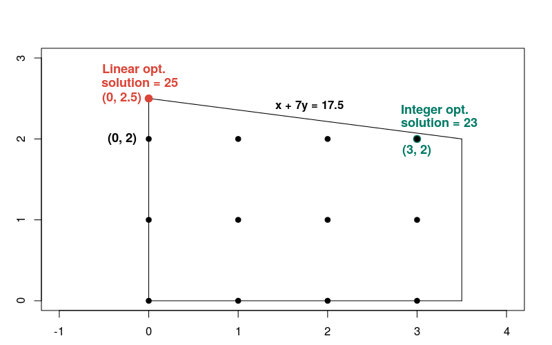
Notice that the integer solution is not close to the linear solution, compared with most other integer points in the feasible region. In general, the solutions to a linear optimization problem and the corresponding integer optimization problems can be far apart. Because of this, the two types of problems require different methods for their solution.