Jump to:
- Control variable overview
- Selecting control variables
- Extract posterior and prior samples of control coefficients
- Including query volume as a control variable
- Using lagged variables
- Population scaling control variables
- Reasons controls don't have causal inference or baseline breakdown
Control variable overview
Controls are variables in the model that aren't treatment variables. Control variables are used to estimate baseline outcome, which is the expected outcome that would occur under the counterfactual scenario where each treatment variable is set to its baseline value for all geos and time periods. (The baseline value is always assigned to zero for media variables, but it is often non-zero for non-media treatments.) Control variables improve estimation of baseline outcome and of the causal effect of treatment variables on the outcome.
Control variables can be classified as follows:
Confounding variables: Have a causal effect on both treatments and the KPI. Including these variables debiases the causal estimates of the treatments on the KPI.
Predictor variables: Have a causal effect on the KPI, but nothing else. Including these variables does nothing to debias the causal effect of treatments. However, strong predictors can reduce the variance of causal estimates.
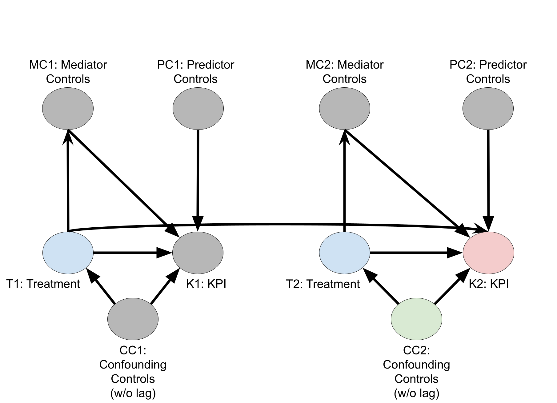
Another variable type is Mediator variables. These are variables that lie in the causal pathway between treatment and KPI. In other words, they have a causal effect on KPI and are causally affected by treatments. Mediator variables shouldn't be included as control variables, because including them will bias causal inference estimates on the treatment variables.
The causal relationships between variable types is explained in the following causal directed acyclic graph (DAG), with the goal of getting the causal effect of media on the KPI. In the names of the nodes, the number 1 denotes variable values at time period 1, the number 2 denotes variable values at time period 2, and so on. The figure only shows nodes for time periods 1 and 2, but assume it continues for \(T\) many time periods.
Selecting control variables
The purpose of marketing mixed modeling (MMM) is causal inference on media effects, not prediction accuracy. So the primary purpose of control variables is to improve inference on the causal effect of treatments on the KPI. It isn't necessary or advisable to include all predictor variables that might improve within-sample or out-of-sample prediction accuracy. Minor improvements in prediction accuracy don't guarantee better causal inference accuracy. Too many predictor variables can inflate the variance of causal estimates and might increase the risk of model misspecification bias.
When brainstorming possible confounding variables to include in the model, practical advice is to focus on identifying variables that affect marketing decisions or that weigh in the mind of decision makers. The rationale is that most variables that affect marketing decisions also have an effect on KPI, and are therefore confounders. Conversely, it is nearly impossible to make a comprehensive list of variables that affect KPI, and such variables are not confounders unless they also affect marketing decisions.
In principle, marketing managers could provide a list of all quantifiable information that was used to make budget decisions, though in reality it might be difficult to compile a complete list. Basic questions to ask marketing managers include:
- At the annual or quarterly level, how did they decide on the total media budget?
- How did they decide the allocation across media channels?
- Within each year, how did they decide the high and low budget weeks?
- Are there any spikes in spend that correspond to certain events, such as holidays or product launches?
- For questions 1-4, what data sources would most strongly correlate with the budget decisions? For example, the previous years' KPI values or economic variables?
- Were there any organic media and what influenced the decision to run the organic media?
- Were there any non-media treatments, such a price changes or promotions, and how did they decide when and how to apply these changes?
Ultimately, our recommendation for control variables is that you:
- Include confounder variables.
- Exclude mediator variables.
- Include strong predictors that can reduce variance of causal estimates.
- Don't include too many variables with the sole purpose of optimizing predictive accuracy because it can increase the risk of model misspecification bias.
Extract posterior and prior samples of control coefficients
Prior and posterior samples of the control coefficients are stored in the Meridian object and can be extracted to create intervals or other summary metrics that can help you determine which controls are relevant.
If the name of the Meridian object is mmm, the prior and posterior
samples for the control coefficients can be found with
mmm.inference_data.prior.gamma_c and mmm.inference_data.posterior.gamma_c
respectively.
Including query volume as a control variable
As mentioned in Selecting control variables, including confounding variables is necessary for debiasing the causal effect of treatments on the KPI. Excluding mediator variables is also necessary for unbiased causal estimates. Query volume might be a mediator for some media channels, but a confounder for other media channels. For example, query volume is certainly a confounder for search ads as a relevant query is often a prerequisite for a search ad. However, other forms of media can drive search behavior, and so query volume is a mediator for those media channels. For more information, see Paid search-modeling.
Since you want to estimate the joint treatment effect of all treatments, you use a single model for inference. So, you must decide either to assume query volume is a confounder and include it in the model, or to assume query volume is a mediator and exclude it from the model. Base your selected assumption on the following considerations:
- The channels that are more important to get unbiased estimates for
- The assumed strengths of relationships between treatments, query volume, and the KPI
- The assumed number of channels where query volume is a confounding variable instead of a mediator variable
We believe that assuming query volume is a confounder, and including it in the model will more often be the right decision due to the relative strength of the relationship between query volume and search media. However, the decision depends on the use case.
Using lagged variables
For certain control variables \(Z\), it can make sense to include lagged values. For example, at each week \(t\), include \(Z_{t-1},\dots ,Z_{t-L}\) for some value of \(L\). We recommend only doing this if you think the lagged values \(t-1, \dots ,t-L\) have a causal effect on the KPI at week \(t\).
When lagged controls aren't needed
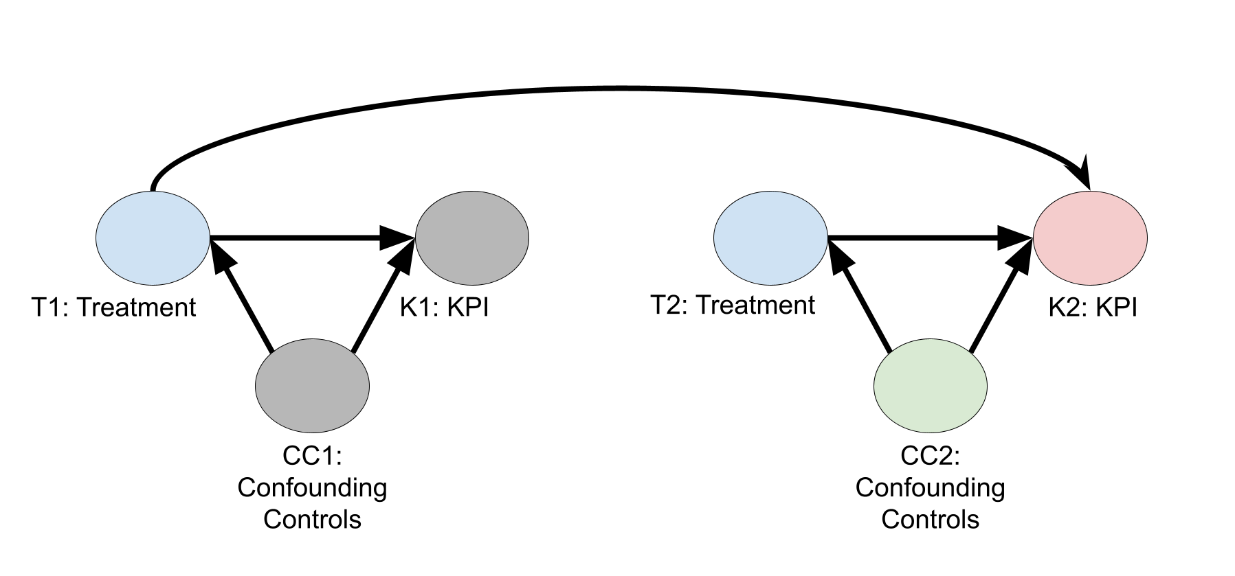
The following diagram shows a causal directed acyclic graph (DAG) where treatments are assumed to have a lagged effect, but controls aren't. Assuming this DAG, lagged controls are not needed. In the names of the nodes, the number 1 denotes variable values at time period 1, the number 2 denotes variable values at time period 2. The figure only shows nodes for time periods 1 and 2, but assume it continues for \(N\) many time periods.
Using the backdoor criteria (Pearl, J. 2009), you can estimate the causal effect of treatments on week 2 KPI by fitting a regression model to estimate \(E\bigl( K2 \big| T2,T1,C2 \bigr) = E\bigl( K2^{(T2, T1)} \big| C2 \bigr)\). Previous controls (\(C1\)) aren't needed.
When lagged controls are needed
The following diagram is a causal DAG where lagged controls are needed. Again, the number in the names of the nodes correspond to the time period. To estimate the causal effect of treatments on week 2 KPI, you must condition on week 1 control variables with a lagged effect on KPI. Failing to do so will leave an unblocked path \(T1 \leftarrow L1 \rightarrow K2\). Utilizing the backdoor criteria, you can fit a regression model to estimate \(E\bigl( K2 \big| T2,T1,C2,L2,L1 \bigr) = E\bigl( K2^{(T2,T1)} \big| C2,L2,L1 \bigr)\).
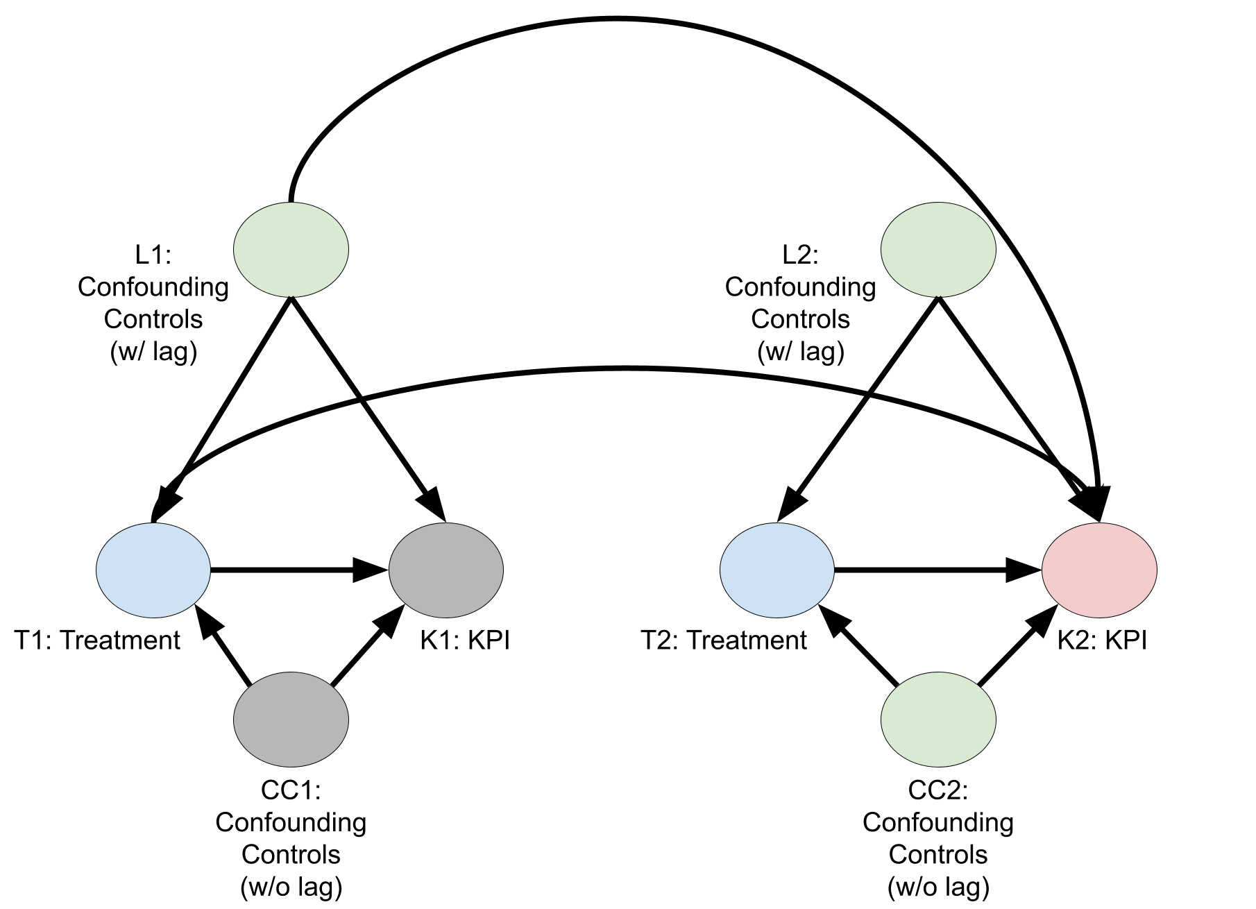
The previous diagram is a simplified 2-week DAG, but in general, for each week \(t\), you should include controls from week \(t,t-1, \dots ,t-L\), where \(L\) is the longest lag where controls are still thought to affect KPI. The value of \(L\) can differ by control variable.
In practice, you can truncate \(L\) at a reasonable value to prevent inflating the model variance by adding too many variables. In many cases, it can be reasonable to ignore lagged controls altogether if the lagged effects are relatively weak. This type of model simplification can be viewed as a bias-variance trade-off.
Population scaling control variables
By default, the KPI and paid and organic media execution are population scaled.
Control variables aren't population scaled by default because some controls,
such as temperature, shouldn't be population scaled. However, some control
variables, such as competitor impressions, should be population-scaled to
maximize their correlation with the population-scaled KPI and with the media
variables. Such variables can be scaled using the
control_population_scaling_id argument in ModelSpec. Similarly, non-media
treatments are not scaled by default. Such variables can be scaled using the
non_media_population_scaling_id in ModelSpec.
Reasons controls don't have causal inference or baseline breakdown
Causal effects and contribution percentages are available for paid media, organic media, and non-media treatments in Meridian. According to the causal graph, the regression effects of these variable types can be interpreted as causal effects. However, the regression effects of control variables cannot be interpreted as causal effects. For this reason, Meridian does not estimate causal effects or contribution percentages for control variables.
Furthermore, Meridian does not decompose baseline outcome into allocation percentages by control variable. Certainly some control variables affect the prediction accuracy of the model more than others. However, this has more to do with the variance each variable contributes to the expected outcome estimates than it does with the additive component of each variable in the expected outcome calculation. It is actually ambiguous as to how a baseline outcome allocation would be defined for control variables. One possible definition could be the change in expected outcome that occurs when each control variable is set to zero for every geo and time period. However, this quantity has no practical meaning because it represents neither the causal effect nor the predictive importance of the control variable. Moreover, a value of zero may not be practically meaningful (or even possible) for every control variable which further obscures the interpretation.
A variable can have a large coefficient and additive component in the expected outcome calculation, and yet have little importance as a predictor of the KPI. This is particularly true for a variable with a low variance. Dropping such a variable from the model could have little impact on the expected outcome estimates if the additive effect can be absorbed into the intercept.
See Organic media and non-media treatment variables for more on these variable types.