Collections can be joined by spatial location as well as by property values. To join based
on spatial location, use a withinDistance() filter with .geo join
fields specified. The .geo field indicates that the item's
geometry is to be used to compute the distance metric. For example, consider the task of
finding all
power plants within 100 kilometers
of Yosemite National Park, USA. For that purpose, use a filter on the geometry
fields, with the maximum distance set to 100 kilometers using the distance
parameter:
// Load a primary collection: protected areas (Yosemite National Park).
var primary = ee.FeatureCollection("WCMC/WDPA/current/polygons")
  .filter(ee.Filter.eq('NAME', 'Yosemite National Park'));

// Load a secondary collection: power plants.
var powerPlants = ee.FeatureCollection('WRI/GPPD/power_plants');

// Define a spatial filter, with distance 100 km.
var distFilter = ee.Filter.withinDistance({
  distance: 100000,
  leftField: '.geo',
  rightField: '.geo',
  maxError: 10
});

// Define a saveAll join.
var distSaveAll = ee.Join.saveAll({
  matchesKey: 'points',
  measureKey: 'distance'
});

// Apply the join.
var spatialJoined = distSaveAll.apply(primary, powerPlants, distFilter);

// Print the result.
print(spatialJoined);
Note that the previous example joins a FeatureCollection to another
FeatureCollection. The saveAll() join sets a property
(points) on each feature in the primary collection which
stores a list of the points within 100 km of the feature. The distance of each point to
the feature is stored in the distance property of each joined point.
Spatial joins can also be used to identify which features
in one collection intersect those in another. For example, consider two feature
collections: a primary collection containing polygons representing the
boundaries of US states, a secondary collection containing point locations
representing power plants. Suppose there is need to determine the number intersecting each
state. This can be accomplished with a spatial join as follows:
// Load the primary collection: US state boundaries.
var states = ee.FeatureCollection('TIGER/2018/States');
// Load the secondary collection: power plants.
var powerPlants = ee.FeatureCollection('WRI/GPPD/power_plants');
// Define a spatial filter as geometries that intersect.
var spatialFilter = ee.Filter.intersects({
leftField: '.geo',
rightField: '.geo',
maxError: 10
});
// Define a save all join.
var saveAllJoin = ee.Join.saveAll({
matchesKey: 'power_plants',
});
// Apply the join.
var intersectJoined = saveAllJoin.apply(states, powerPlants, spatialFilter);
// Add power plant count per state as a property.
intersectJoined = intersectJoined.map(function(state) {
// Get "power_plant" intersection list, count how many intersected this state.
var nPowerPlants = ee.List(state.get('power_plants')).size();
// Return the state feature with a new property: power plant count.
return state.set('n_power_plants', nPowerPlants);
});
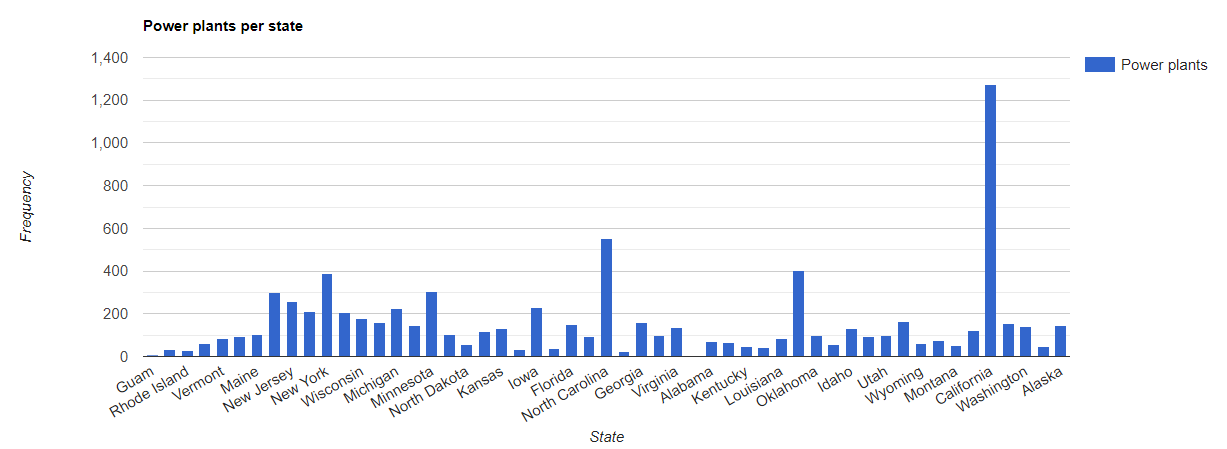
// Make a bar chart for the number of power plants per state.
var chart = ui.Chart.feature.byFeature(intersectJoined, 'NAME', 'n_power_plants')
.setChartType('ColumnChart')
.setSeriesNames({n_power_plants: 'Power plants'})
.setOptions({
title: 'Power plants per state',
hAxis: {title: 'State'},
vAxis: {title: 'Frequency'}});
// Print the chart to the console.
print(chart);
In the previous example, note that the intersects() filter doesn’t store
a distance as the withinDistance() filter does. The output should look
something like Figure 1.