इस पेज का अनुवाद Cloud Translation API से किया गया है.

फिर से सैंपलिंग करना और रिज़ॉल्यूशन कम करना

जैसा कि प्रोजेक्शंस दस्तावेज़ में बताया गया है, Earth Engine, फिर से प्रोजेक्ट करने के दौरान डिफ़ॉल्ट रूप से, नियरेस्ट नेबर रीसैंपलिंग करता है. resample() या reduceResolution() तरीकों से, इस व्यवहार को बदला जा सकता है. खास तौर पर, जब इनमें से कोई एक तरीका किसी इनपुट इमेज पर लागू किया जाता है, तो इनपुट का ज़रूरी रीप्रोजेक्शन, बताए गए रीसैंपलिंग या एग्रीगेशन तरीके का इस्तेमाल करके किया जाएगा.

फिर से सैंपलिंग करना

resample() से, अगले बार प्रॉजेक्ट करते समय, रेसैंपलिंग के लिए बताए गए तरीके ('bilinear' या 'bicubic') का इस्तेमाल किया जाता है. इनपुट का अनुरोध, आउटपुट प्रोजेक्शन में किया जाता है. इसलिए, इनपुट पर किसी भी अन्य कार्रवाई से पहले, इनपुट को फिर से प्रोजेक्ट किया जा सकता है. इस वजह से, सीधे इनपुट इमेज पर resample() को कॉल करें. इस आसान उदाहरण पर ध्यान दें:

कोड एडिटर (JavaScript)

// Load a Landsat image over San Francisco, California, UAS.
var landsat = ee.Image('LANDSAT/LC08/C02/T1_TOA/LC08_044034_20160323');

// Set display and visualization parameters.
Map.setCenter(-122.37383, 37.6193, 15);
var visParams = {bands: ['B4', 'B3', 'B2'], max: 0.3};

// Display the Landsat image using the default nearest neighbor resampling.
// when reprojecting to Mercator for the Code Editor map.
Map.addLayer(landsat, visParams, 'original image');

// Force the next reprojection on this image to use bicubic resampling.
var resampled = landsat.resample('bicubic');

// Display the Landsat image using bicubic resampling.
Map.addLayer(resampled, visParams, 'resampled');

Python सेटअप

Python API के बारे में जानकारी पाने और इंटरैक्टिव डेवलपमेंट के लिए geemap का इस्तेमाल करने के लिए, Python एनवायरमेंट पेज देखें.

import ee
import geemap.core as geemap

Colab (Python)

# Load a Landsat image over San Francisco, California, UAS.
landsat = ee.Image('LANDSAT/LC08/C02/T1_TOA/LC08_044034_20160323')

# Set display and visualization parameters.
m = geemap.Map()
m.set_center(-122.37383, 37.6193, 15)
vis_params = {'bands': ['B4', 'B3', 'B2'], 'max': 0.3}

# Display the Landsat image using the default nearest neighbor resampling.
# when reprojecting to Mercator for the Code Editor map.
m.add_layer(landsat, vis_params, 'original image')

# Force the next reprojection on this image to use bicubic resampling.
resampled = landsat.resample('bicubic')

# Display the Landsat image using bicubic resampling.
m.add_layer(resampled, vis_params, 'resampled')

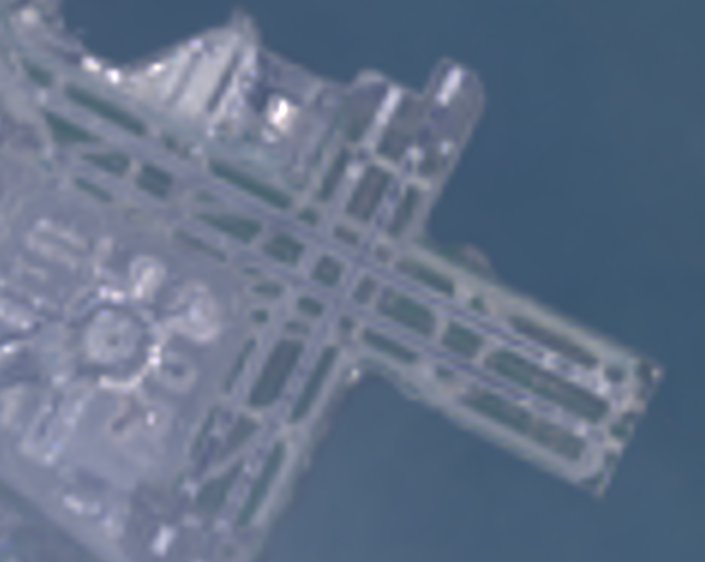
ध्यान दें कि 'bicubic' रीसैंपलिंग की वजह से, आउटपुट पिक्सल, ओरिजनल इमेज (पहली इमेज) के मुकाबले ज़्यादा स्मूद दिखते हैं.

**पहली इमेज.** नियरेस्ट नेबर तकनीक का इस्तेमाल करके, Landsat इमेज को फिर से सैंपल किया गया.

इस कोड सैंपल के लिए ऑपरेशन का क्रम, दूसरे चित्र में डायग्राम के तौर पर दिखाया गया है. खास तौर पर, maps Mercator प्रोजेक्शन में, इनपुट इमेज पर बताए गए रीसैंपलिंग तरीके के साथ, इमेज को फिर से प्रोजेक्ट किया जाता है.

कार्रवाइयों का फ़्लो चार्ट

दूसरी इमेज. कोड एडिटर में दिखाने से पहले, इनपुट इमेज पर resample() को कॉल करने पर होने वाली प्रोसेस का फ़्लो चार्ट. घुमावदार लाइनें, फिर से प्रोजेक्ट करने के लिए जानकारी के फ़्लो को दिखाती हैं: खास तौर पर, आउटपुट प्रोजेक्शन, स्केल, और फिर से सैंपलिंग करने के तरीके का इस्तेमाल करना.

रिज़ॉल्यूशन कम करना

मान लें कि आपका लक्ष्य, फिर से प्रोजेक्ट करने के दौरान फिर से सैंपलिंग करने के बजाय, किसी दूसरे प्रोजेक्शन में पिक्सल को बड़े पिक्सल में एग्रीगेट करना है. यह अलग-अलग स्केल पर इमेज डेटासेट की तुलना करने के लिए मददगार होता है. उदाहरण के लिए, Landsat-आधारित प्रॉडक्ट के 30 मीटर पिक्सल से लेकर MODIS-आधारित प्रॉडक्ट के कोर्स पिक्सल (ज़्यादा स्केल) तक. reduceResolution() तरीके से, डेटा इकट्ठा करने की इस प्रोसेस को कंट्रोल किया जा सकता है. resample() की तरह ही, इनपुट पर reduceResolution() को कॉल करें, ताकि इमेज के अगले रीप्रोजेक्टेशन पर असर पड़े. यहां दिए गए उदाहरण में, reduceResolution() का इस्तेमाल करके, 30 मीटर रिज़ॉल्यूशन पर मौजूद वन कवर डेटा की तुलना, 500 मीटर रिज़ॉल्यूशन पर मौजूद वनस्पति सूचकांक से की गई है:

कोड एडिटर (JavaScript)

// Load a MODIS EVI image.
var modis = ee.Image(ee.ImageCollection('MODIS/061/MOD13A1').first())
    .select('EVI');

// Display the EVI image near La Honda, California.
Map.setCenter(-122.3616, 37.5331, 12);
Map.addLayer(modis, {min: 2000, max: 5000}, 'MODIS EVI');

// Get information about the MODIS projection.
var modisProjection = modis.projection();
print('MODIS projection:', modisProjection);

// Load and display forest cover data at 30 meters resolution.
var forest = ee.Image('UMD/hansen/global_forest_change_2023_v1_11')
    .select('treecover2000');
Map.addLayer(forest, {max: 80}, 'forest cover 30 m');

// Get the forest cover data at MODIS scale and projection.
var forestMean = forest
    // Force the next reprojection to aggregate instead of resampling.
    .reduceResolution({
      reducer: ee.Reducer.mean(),
      maxPixels: 1024
    })
    // Request the data at the scale and projection of the MODIS image.
    .reproject({
      crs: modisProjection
    });

// Display the aggregated, reprojected forest cover data.
Map.addLayer(forestMean, {max: 80}, 'forest cover at MODIS scale');

Python सेटअप

import ee
import geemap.core as geemap

Colab (Python)

# Load a MODIS EVI image.
modis = ee.Image(ee.ImageCollection('MODIS/006/MOD13A1').first()).select('EVI')

# Display the EVI image near La Honda, California.
m.set_center(-122.3616, 37.5331, 12)
m.add_layer(modis, {'min': 2000, 'max': 5000}, 'MODIS EVI')

# Get information about the MODIS projection.
modis_projection = modis.projection()
display('MODIS projection:', modis_projection)

# Load and display forest cover data at 30 meters resolution.
forest = ee.Image('UMD/hansen/global_forest_change_2015').select(
    'treecover2000'
)
m.add_layer(forest, {'max': 80}, 'forest cover 30 m')

# Get the forest cover data at MODIS scale and projection.
forest_mean = (
    forest
    # Force the next reprojection to aggregate instead of resampling.
    .reduceResolution(reducer=ee.Reducer.mean(), maxPixels=1024)
    # Request the data at the scale and projection of the MODIS image.
    .reproject(crs=modis_projection)
)

# Display the aggregated, reprojected forest cover data.
m.add_layer(forest_mean, {'max': 80}, 'forest cover at MODIS scale')

इस उदाहरण में, ध्यान दें कि आउटपुट प्रोजेक्शन को साफ़ तौर पर reproject() के साथ सेट किया गया है. MODIS सिनसॉइडल प्रोजेक्शन में फिर से प्रोजेक्ट करने के दौरान, छोटे पिक्सल को फिर से सैंपल करने के बजाय, तय किए गए रिड्यूसर (उदाहरण में ee.Reducer.mean()) के साथ एग्रीगेट किया जाता है. ऑपरेशन का यह क्रम, तीसरे चित्र में दिखाया गया है. हालांकि, इस उदाहरण में reduceResolution() के असर को विज़ुअलाइज़ करने के लिए reproject() का इस्तेमाल किया गया है, लेकिन ज़्यादातर स्क्रिप्ट को साफ़ तौर पर फिर से प्रोजेक्ट करने की ज़रूरत नहीं होती. चेतावनी देखने के लिए यहां जाएं.

कार्रवाइयों का फ़्लो चार्ट

तीसरी इमेज. reproject() से पहले किसी इनपुट इमेज पर reduceResolution() को कॉल करने पर, कार्रवाइयों का फ़्लो चार्ट. घुमावदार लाइनें, फिर से प्रोजेक्ट करने के लिए जानकारी के फ़्लो को दिखाती हैं: खास तौर पर, आउटपुट प्रोजेक्शन, स्केल, और इस्तेमाल किए जाने वाले पिक्सल एग्रीगेशन का तरीका.

साफ़ तौर पर reproject() की ज़रूरत पड़े.

`ReduceResolution` के लिए पिक्सल वेट

reduceResolution() एग्रीगेशन प्रोसेस के दौरान इस्तेमाल किए गए पिक्सल के वज़न, एग्रीगेट किए जा रहे छोटे पिक्सल और आउटपुट प्रोजेक्शन के ज़रिए तय किए गए बड़े पिक्सल के ओवरलैप पर आधारित होते हैं. इसे चौथे चित्र में दिखाया गया है.

इनपुट और आउटपुट पिक्सल

चौथी इमेज. reduceResolution() के लिए इनपुट पिक्सल (काले) और आउटपुट पिक्सल (नीले).

डिफ़ॉल्ट रूप से, इनपुट पिक्सल के वज़न का हिसाब, इनपुट पिक्सल के ज़रिए कवर किए गए आउटपुट पिक्सल एरिया के फ़्रैक्शन के तौर पर लगाया जाता है. डायग्राम में, आउटपुट पिक्सल का क्षेत्रफल a है. इंटरसेक्शन एरिया b वाले इनपुट पिक्सल का वज़न b/a के तौर पर कैलकुलेट किया जाता है. साथ ही, इंटरसेक्शन एरिया c वाले इनपुट पिक्सल का वज़न c/a के तौर पर कैलकुलेट किया जाता है. इस वजह से, मीन रिड्यूसर के अलावा किसी दूसरे रिड्यूसर का इस्तेमाल करने पर, अनचाहे नतीजे मिल सकते हैं. उदाहरण के लिए, हर पिक्सल में जंगल के क्षेत्र का हिसाब लगाने के लिए, पिक्सल के कवर किए गए हिस्से का हिसाब लगाने के लिए, मीन रिड्यूसर का इस्तेमाल करें. इसके बाद, क्षेत्र से गुणा करें. इसके बजाय, छोटे पिक्सल में क्षेत्र का हिसाब लगाकर, उन्हें सम रिड्यूसर की मदद से जोड़ें:

कोड एडिटर (JavaScript)

// Compute forest area per MODIS pixel.
var forestArea = forest.gt(0)
    // Force the next reprojection to aggregate instead of resampling.
    .reduceResolution({
      reducer: ee.Reducer.mean(),
      maxPixels: 1024
    })
    // The reduce resolution returns the fraction of the MODIS pixel
    // that's covered by 30 meter forest pixels.  Convert to area
    // after the reduceResolution() call.
    .multiply(ee.Image.pixelArea())
    // Request the data at the scale and projection of the MODIS image.
    .reproject({
      crs: modisProjection
    });
Map.addLayer(forestArea, {max: 500 * 500}, 'forested area at MODIS scale');

Python सेटअप

import ee
import geemap.core as geemap

Colab (Python)

# Compute forest area per MODIS pixel.
forest_area = (
    forest.gt(0)
    # Force the next reprojection to aggregate instead of resampling.
    .reduceResolution(reducer=ee.Reducer.mean(), maxPixels=1024)
    # The reduce resolution returns the fraction of the MODIS pixel
    # that's covered by 30 meter forest pixels.  Convert to area
    # after the reduceResolution() call.
    .multiply(ee.Image.pixelArea())
    # Request the data at the scale and projection of the MODIS image.
    .reproject(crs=modis_projection)
)
m.add_layer(forest_area, {'max': 500 * 500}, 'forested area at MODIS scale')
m