सूचना: जिन गैर-व्यावसायिक प्रोजेक्ट के लिए Earth Engine को 15 अप्रैल, 2025 से पहले रजिस्टर किया गया है उन्हें ऐक्सेस बनाए रखने के लिए, गैर-व्यावसायिक इस्तेमाल से जुड़ी ज़रूरी शर्तों की पुष्टि करनी होगी. अगर आपने 26 सितंबर, 2025 तक पुष्टि नहीं की, तो आपके ऐक्सेस को होल्ड पर रखा जा सकता है.

इस पेज का अनुवाद Cloud Translation API से किया गया है.

लीनियर रिग्रेशन

Earth Engine में, रिड्यूसर का इस्तेमाल करके लीनियर रिग्रेशन करने के कई तरीके हैं:

ee.Reducer.linearFit()
ee.Reducer.linearRegression()
ee.Reducer.robustLinearRegression()
ee.Reducer.ridgeRegression()

सबसे आसान लीनियर रिग्रेशन रिड्यूसर linearFit() है, जो एक वैरिएबल के लीनियर फ़ंक्शन के लिए, कम से कम स्क्वेयर का अनुमान लगाता है. इसमें एक स्थिर शब्द होता है. लीनियर मॉडलिंग के लिए ज़्यादा सुविधाजनक तरीके का इस्तेमाल करने के लिए, उनमें से किसी एक का इस्तेमाल करें लीनियर रिग्रेशन रिड्यूसर, जो इंडिपेंडेंट और डिपेंडेंट वैरिएबल की वैरिएबल संख्या की अनुमति देते हैं. linearRegression(), ऑर्डिनरी लीस्ट स्क्वेयर रिग्रेशन(ओएलएस) लागू करता है. robustLinearRegression(), डेटा में मौजूद आउटलायर की वैल्यू को बार-बार कम करने के लिए, रिग्रेशन अवशेष पर आधारित लागत फ़ंक्शन का इस्तेमाल करता है (O’Leary, 1990). ridgeRegression(), L2 रेगुलराइज़ेशन के साथ लीनियर रिग्रेशन करता है.

इन तरीकों से किया जाने वाला रिग्रेशन ऐनलिसिस, ee.ImageCollection, ee.Image, ee.FeatureCollection, और ee.List ऑब्जेक्ट को कम करने के लिए सही है. नीचे दिए गए उदाहरणों में, हर एक के लिए एक ऐप्लिकेशन दिखाया गया है. ध्यान दें कि linearRegression(), robustLinearRegression(), और ridgeRegression() के इनपुट और आउटपुट का स्ट्रक्चर एक जैसा है. हालांकि, linearFit() के लिए दो-बैंड वाला इनपुट (X के बाद Y) चाहिए. साथ ही, ridgeRegression() में एक अतिरिक्त पैरामीटर (lambda, ज़रूरी नहीं) और आउटपुट (pValue) है.

ee.ImageCollection

`linearFit()`

डेटा को दो-बैंड वाली इनपुट इमेज के तौर पर सेट अप किया जाना चाहिए. इसमें पहला बैंड, स्वतंत्र वैरिएबल और दूसरा बैंड, आश्रित वैरिएबल होता है. यहां दिए गए उदाहरण में, आने वाले समय में होने वाली बारिश के लीनियर रुझान का अनुमान दिखाया गया है. यह अनुमान, जलवायु मॉडल के आधार पर NEX-DCP30 डेटा में, 2006 के बाद के डेटा के लिए लगाया गया है. डिपेंडेंट वैरिएबल, अनुमानित बारिश है और इंडिपेंडेंट वैरिएबल, समय है. इसे linearFit() को कॉल करने से पहले जोड़ा गया है:

कोड एडिटर (JavaScript)

// This function adds a time band to the image.
var createTimeBand = function(image) {
  // Scale milliseconds by a large constant to avoid very small slopes
  // in the linear regression output.
  return image.addBands(image.metadata('system:time_start').divide(1e18));
};

// Load the input image collection: projected climate data.
var collection = ee.ImageCollection('NASA/NEX-DCP30_ENSEMBLE_STATS')
  .filter(ee.Filter.eq('scenario', 'rcp85'))
  .filterDate(ee.Date('2006-01-01'), ee.Date('2050-01-01'))
  // Map the time band function over the collection.
  .map(createTimeBand);

// Reduce the collection with the linear fit reducer.
// Independent variable are followed by dependent variables.
var linearFit = collection.select(['system:time_start', 'pr_mean'])
  .reduce(ee.Reducer.linearFit());

// Display the results.
Map.setCenter(-100.11, 40.38, 5);
Map.addLayer(linearFit,
  {min: 0, max: [-0.9, 8e-5, 1], bands: ['scale', 'offset', 'scale']}, 'fit');

ध्यान दें कि आउटपुट में दो बैंड होते हैं, 'ऑफ़सेट' (इंटरसेप्ट) और 'स्केल' (इस संदर्भ में 'स्केल' का मतलब लाइन के स्लोप से है और इसे कई रिड्यूसर में स्केल पैरामीटर इनपुट के साथ नहीं जोड़ा जाना चाहिए, जो कि स्पेस स्केल है). इसकी वजह से, आपको 'ट्रेंड में बढ़ोतरी' वाले इलाके नीले रंग में, 'ट्रेंड में गिरावट' वाले इलाके लाल रंग में, और 'ट्रेंड में कोई बदलाव नहीं' वाले इलाके हरे रंग में दिखेंगे. यह नतीजा, पहली इमेज की तरह दिखेगा.

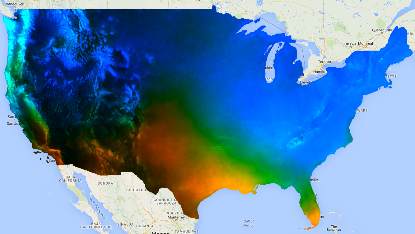
पहली इमेज. अनुमानित बारिश पर लागू किया गया linearFit() का आउटपुट. जिन इलाकों में बारिश या बर्फ़बारी की मात्रा बढ़ने का अनुमान है उन्हें नीले रंग में दिखाया जाता है. वहीं, जिन इलाकों में बारिश या बर्फ़बारी की मात्रा कम होने का अनुमान है उन्हें लाल रंग में दिखाया जाता है.

`linearRegression()`

उदाहरण के लिए, मान लें कि दो डिपेंडेंट वैरिएबल हैं: बारिश और सबसे ज़्यादा तापमान. साथ ही, दो इंडिपेंडेंट वैरिएबल हैं: एक कॉन्स्टेंट और समय. यह कलेक्शन, पिछले उदाहरण जैसा ही है. हालांकि, डेटा को कम करने से पहले, कॉन्स्टेंट बैंड को मैन्युअल तरीके से जोड़ना होगा. इनपुट के पहले दो बैंड, 'X' (इंडिपेंडेंट) वैरिएबल होते हैं और अगले दो बैंड, 'Y' (डिपेंडेंट) वैरिएबल होते हैं. इस उदाहरण में, पहले रिग्रेशन कोएफ़िशिएंट पाएं. इसके बाद, अपनी पसंद के बैंड निकालने के लिए, ऐरे इमेज को फ़्लैट करें:

कोड एडिटर (JavaScript)

// This function adds a time band to the image.
var createTimeBand = function(image) {
  // Scale milliseconds by a large constant.
  return image.addBands(image.metadata('system:time_start').divide(1e18));
};

// This function adds a constant band to the image.
var createConstantBand = function(image) {
  return ee.Image(1).addBands(image);
};

// Load the input image collection: projected climate data.
var collection = ee.ImageCollection('NASA/NEX-DCP30_ENSEMBLE_STATS')
  .filterDate(ee.Date('2006-01-01'), ee.Date('2099-01-01'))
  .filter(ee.Filter.eq('scenario', 'rcp85'))
  // Map the functions over the collection, to get constant and time bands.
  .map(createTimeBand)
  .map(createConstantBand)
  // Select the predictors and the responses.
  .select(['constant', 'system:time_start', 'pr_mean', 'tasmax_mean']);

// Compute ordinary least squares regression coefficients.
var linearRegression = collection.reduce(
  ee.Reducer.linearRegression({
    numX: 2,
    numY: 2
}));

// Compute robust linear regression coefficients.
var robustLinearRegression = collection.reduce(
  ee.Reducer.robustLinearRegression({
    numX: 2,
    numY: 2
}));

// The results are array images that must be flattened for display.
// These lists label the information along each axis of the arrays.
var bandNames = [['constant', 'time'], // 0-axis variation.
                 ['precip', 'temp']]; // 1-axis variation.

// Flatten the array images to get multi-band images according to the labels.
var lrImage = linearRegression.select(['coefficients']).arrayFlatten(bandNames);
var rlrImage = robustLinearRegression.select(['coefficients']).arrayFlatten(bandNames);

// Display the OLS results.
Map.setCenter(-100.11, 40.38, 5);
Map.addLayer(lrImage,
  {min: 0, max: [-0.9, 8e-5, 1], bands: ['time_precip', 'constant_precip', 'time_precip']}, 'OLS');

// Compare the results at a specific point:
print('OLS estimates:', lrImage.reduceRegion({
  reducer: ee.Reducer.first(),
  geometry: ee.Geometry.Point([-96.0, 41.0]),
  scale: 1000
}));

print('Robust estimates:', rlrImage.reduceRegion({
  reducer: ee.Reducer.first(),
  geometry: ee.Geometry.Point([-96.0, 41.0]),
  scale: 1000
}));

नतीजों की जांच करके पता लगाएं कि linearRegression() आउटपुट, linearFit() रिड्यूसर के अनुमानित गुणांक के बराबर है. हालांकि, linearRegression() आउटपुट में, अन्य डिपेंडेंट वैरिएबल tasmax_mean के लिए भी गुणांक होते हैं. बेहतर लीनियर रिग्रेशन के गुणांक, ओएलएस के अनुमान से अलग होते हैं. इस उदाहरण में, किसी खास पॉइंट पर अलग-अलग रिग्रेशन के तरीकों के कोएफ़िशिएंट की तुलना की गई है.

ee.Image

ee.Image ऑब्जेक्ट के संदर्भ में, क्षेत्र के पिक्सल पर लीनियर रिग्रेशन करने के लिए, रिग्रेशन रिड्यूसर का इस्तेमाल reduceRegion या reduceRegions के साथ किया जा सकता है. यहां दिए गए उदाहरणों में, किसी पॉलीगॉन में Landsat बैंड के बीच रिग्रेशन कोएफ़िशिएंट का हिसाब लगाने का तरीका बताया गया है.

`linearFit()`

ऐरे डेटा चार्ट के बारे में बताने वाले गाइड सेक्शन में, Landsat 8 SWIR1 और SWIR2 बैंड के बीच के संबंध का स्कैटर प्लॉट दिखाया गया है. यहां, इस संबंध के लिए लीनियर रिग्रेशन गुणांक का हिसाब लगाया जाता है. 'offset' (y-इंटरसेप्ट) और 'scale' (ढलान) प्रॉपर्टी वाली एक डिक्शनरी दिखाती है.

कोड एडिटर (JavaScript)

// Define a rectangle geometry around San Francisco.
var sanFrancisco = ee.Geometry.Rectangle([-122.45, 37.74, -122.4, 37.8]);

// Import a Landsat 8 TOA image for this region.
var img = ee.Image('LANDSAT/LC08/C02/T1_TOA/LC08_044034_20140318');

// Subset the SWIR1 and SWIR2 bands. In the regression reducer, independent
// variables come first followed by the dependent variables. In this case,
// B5 (SWIR1) is the independent variable and B6 (SWIR2) is the dependent
// variable.
var imgRegress = img.select(['B5', 'B6']);

// Calculate regression coefficients for the set of pixels intersecting the
// above defined region using reduceRegion with ee.Reducer.linearFit().
var linearFit = imgRegress.reduceRegion({
  reducer: ee.Reducer.linearFit(),
  geometry: sanFrancisco,
  scale: 30,
});

// Inspect the results.
print('OLS estimates:', linearFit);
print('y-intercept:', linearFit.get('offset'));
print('Slope:', linearFit.get('scale'));

`linearRegression()`

यहां पिछले linearFit सेक्शन का वही विश्लेषण लागू किया गया है. हालांकि, इस बार ee.Reducer.linearRegression फ़ंक्शन का इस्तेमाल किया गया है. ध्यान दें कि रिग्रेशन इमेज, तीन अलग-अलग इमेज से बनाई जाती है: एक स्थिर इमेज और एक ही लैंडसैट 8 इमेज से SWIR1 और SWIR2 बैंड दिखाने वाली इमेज. ध्यान रखें कि ee.Reducer.linearRegression के हिसाब से क्षेत्र को छोटा करने के लिए, इनपुट इमेज बनाने के लिए बैंड के किसी भी सेट को जोड़ा जा सकता है. इसके लिए, यह ज़रूरी नहीं है कि वे एक ही सोर्स इमेज से हों.

कोड एडिटर (JavaScript)

// Define a rectangle geometry around San Francisco.
var sanFrancisco = ee.Geometry.Rectangle([-122.45, 37.74, -122.4, 37.8]);

// Import a Landsat 8 TOA image for this region.
var img = ee.Image('LANDSAT/LC08/C02/T1_TOA/LC08_044034_20140318');

// Create a new image that is the concatenation of three images: a constant,
// the SWIR1 band, and the SWIR2 band.
var constant = ee.Image(1);
var xVar = img.select('B5');
var yVar = img.select('B6');
var imgRegress = ee.Image.cat(constant, xVar, yVar);

// Calculate regression coefficients for the set of pixels intersecting the
// above defined region using reduceRegion. The numX parameter is set as 2
// because the constant and the SWIR1 bands are independent variables and they
// are the first two bands in the stack; numY is set as 1 because there is only
// one dependent variable (SWIR2) and it follows as band three in the stack.
var linearRegression = imgRegress.reduceRegion({
  reducer: ee.Reducer.linearRegression({
    numX: 2,
    numY: 1
  }),
  geometry: sanFrancisco,
  scale: 30,
});

// Convert the coefficients array to a list.
var coefList = ee.Array(linearRegression.get('coefficients')).toList();

// Extract the y-intercept and slope.
var b0 = ee.List(coefList.get(0)).get(0); // y-intercept
var b1 = ee.List(coefList.get(1)).get(0); // slope

// Extract the residuals.
var residuals = ee.Array(linearRegression.get('residuals')).toList().get(0);

// Inspect the results.
print('OLS estimates', linearRegression);
print('y-intercept:', b0);
print('Slope:', b1);
print('Residuals:', residuals);

'coefficients' और 'residuals' प्रॉपर्टी वाली एक डिक्शनरी दिखाई जाती है. 'coefficients' प्रॉपर्टी, डाइमेंशन (numX, numY) वाला एक कलेक्शन है. हर कॉलम में, उससे जुड़े डिपेंडेंट वैरिएबल के लिए कोएफ़िशिएंट होते हैं. इस मामले में, ऐरे में दो पंक्तियां और एक कॉलम है; पहली पंक्ति, पहला कॉलम y-इंटरसेप्ट है और दूसरी पंक्ति, पहला कॉलम ढलान है. 'residuals' प्रॉपर्टी, हर डिपेंडेंट वैरिएबल के अवशेषों के रूट मीन स्क्वेयर का वेक्टर होती है. नतीजे को अरे के तौर पर कास्ट करके, कॉफ़िशिएंट निकालें. इसके बाद, अपनी पसंद के एलिमेंट को स्लाइस करें या अरे को सूची में बदलें और इंडेक्स पोज़िशन के हिसाब से कॉफ़िशिएंट चुनें.

ee.FeatureCollection

मान लें कि आपको Sentinel-2 और Landsat 8 SWIR1 रिफ़्लेक्शन के बीच का लीनियर संबंध जानना है. इस उदाहरण में, पॉइंट के फ़ीचर कलेक्शन के तौर पर फ़ॉर्मैट किए गए पिक्सल के एक रैंडम सैंपल का इस्तेमाल, संबंध का हिसाब लगाने के लिए किया जाता है. पिक्सल पेयर का स्कैटर प्लॉट और सबसे अच्छी फ़िट वाली कम से कम स्क्वेयर्स वाली रेखा जनरेट की जाती है (पहला फ़ोटो).

कोड एडिटर (JavaScript)

// Import a Sentinel-2 TOA image.
var s2ImgSwir1 = ee.Image('COPERNICUS/S2/20191022T185429_20191022T185427_T10SEH');

// Import a Landsat 8 TOA image from 12 days earlier than the S2 image.
var l8ImgSwir1 = ee.Image('LANDSAT/LC08/C02/T1_TOA/LC08_044033_20191010');

// Get the intersection between the two images - the area of interest (aoi).
var aoi = s2ImgSwir1.geometry().intersection(l8ImgSwir1.geometry());

// Get a set of 1000 random points from within the aoi. A feature collection
// is returned.
var sample = ee.FeatureCollection.randomPoints({
  region: aoi,
  points: 1000
});

// Combine the SWIR1 bands from each image into a single image.
var swir1Bands = s2ImgSwir1.select('B11')
  .addBands(l8ImgSwir1.select('B6'))
  .rename(['s2_swir1', 'l8_swir1']);

// Sample the SWIR1 bands using the sample point feature collection.
var imgSamp = swir1Bands.sampleRegions({
  collection: sample,
  scale: 30
})
// Add a constant property to each feature to be used as an independent variable.
.map(function(feature) {
  return feature.set('constant', 1);
});

// Compute linear regression coefficients. numX is 2 because
// there are two independent variables: 'constant' and 's2_swir1'. numY is 1
// because there is a single dependent variable: 'l8_swir1'. Cast the resulting
// object to an ee.Dictionary for easy access to the properties.
var linearRegression = ee.Dictionary(imgSamp.reduceColumns({
  reducer: ee.Reducer.linearRegression({
    numX: 2,
    numY: 1
  }),
  selectors: ['constant', 's2_swir1', 'l8_swir1']
}));

// Convert the coefficients array to a list.
var coefList = ee.Array(linearRegression.get('coefficients')).toList();

// Extract the y-intercept and slope.
var yInt = ee.List(coefList.get(0)).get(0); // y-intercept
var slope = ee.List(coefList.get(1)).get(0); // slope

// Gather the SWIR1 values from the point sample into a list of lists.
var props = ee.List(['s2_swir1', 'l8_swir1']);
var regressionVarsList = ee.List(imgSamp.reduceColumns({
  reducer: ee.Reducer.toList().repeat(props.size()),
  selectors: props
}).get('list'));

// Convert regression x and y variable lists to an array - used later as input
// to ui.Chart.array.values for generating a scatter plot.
var x = ee.Array(ee.List(regressionVarsList.get(0)));
var y1 = ee.Array(ee.List(regressionVarsList.get(1)));

// Apply the line function defined by the slope and y-intercept of the
// regression to the x variable list to create an array that will represent
// the regression line in the scatter plot.
var y2 = ee.Array(ee.List(regressionVarsList.get(0)).map(function(x) {
  var y = ee.Number(x).multiply(slope).add(yInt);
  return y;
}));

// Concatenate the y variables (Landsat 8 SWIR1 and predicted y) into an array
// for input to ui.Chart.array.values for plotting a scatter plot.
var yArr = ee.Array.cat([y1, y2], 1);

// Make a scatter plot of the two SWIR1 bands for the point sample and include
// the least squares line of best fit through the data.
print(ui.Chart.array.values({
  array: yArr,
  axis: 0,
  xLabels: x})
  .setChartType('ScatterChart')
  .setOptions({
    legend: {position: 'none'},
    hAxis: {'title': 'Sentinel-2 SWIR1'},
    vAxis: {'title': 'Landsat 8 SWIR1'},
    series: {
      0: {
        pointSize: 0.2,
        dataOpacity: 0.5,
      },
      1: {
        pointSize: 0,
        lineWidth: 2,
      }
    }
  })
);

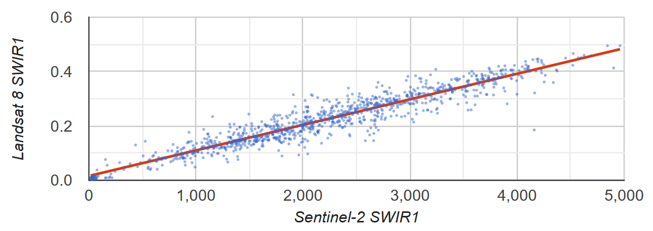
दूसरी इमेज. पिक्सल के सैंपल के लिए स्कैटर प्लॉट और सबसे कम स्क्वेयर वाली लीनियर रिग्रेशन लाइन, जो Sentinel-2 और Landsat 8 SWIR1 TOA रिफ़्लेक्शन दिखाती है.

ee.List

2-D ee.List ऑब्जेक्ट के कॉलम, रिग्रेशन रिड्यूसर के इनपुट हो सकते हैं. नीचे दिए गए उदाहरणों में, इस बात के आसान सबूत दिए गए हैं कि इंडिपेंडेंट वैरिएबल, डिपेंडेंट वैरिएबल की कॉपी होता है. इससे y-इंटरसेप्ट 0 और स्लोप 1 होता है.

`linearFit()`

कोड एडिटर (JavaScript)

// Define a list of lists, where columns represent variables. The first column
// is the independent variable and the second is the dependent variable.
var listsVarColumns = ee.List([
  [1, 1],
  [2, 2],
  [3, 3],
  [4, 4],
  [5, 5]
]);

// Compute the least squares estimate of a linear function. Note that an
// object is returned; cast it as an ee.Dictionary to make accessing the
// coefficients easier.
var linearFit = ee.Dictionary(listsVarColumns.reduce(ee.Reducer.linearFit()));

// Inspect the result.
print(linearFit);
print('y-intercept:', linearFit.get('offset'));
print('Slope:', linearFit.get('scale'));

अगर वैरिएबल को पंक्तियों में दिखाया गया है, तो सूची को ट्रांसपोज़ करें. इसके लिए, सूची को ee.Array में बदलें, फिर उसे ट्रांसपोज़ करें और फिर से ee.List में बदलें.

कोड एडिटर (JavaScript)

// If variables in the list are arranged as rows, you'll need to transpose it.
// Define a list of lists where rows represent variables. The first row is the
// independent variable and the second is the dependent variable.
var listsVarRows = ee.List([
  [1, 2, 3, 4, 5],
  [1, 2, 3, 4, 5]
]);

// Cast the ee.List as an ee.Array, transpose it, and cast back to ee.List.
var listsVarColumns = ee.Array(listsVarRows).transpose().toList();

// Compute the least squares estimate of a linear function. Note that an
// object is returned; cast it as an ee.Dictionary to make accessing the
// coefficients easier.
var linearFit = ee.Dictionary(listsVarColumns.reduce(ee.Reducer.linearFit()));

// Inspect the result.
print(linearFit);
print('y-intercept:', linearFit.get('offset'));
print('Slope:', linearFit.get('scale'));

`linearRegression()`

ee.Reducer.linearRegression() का इस्तेमाल, ऊपर दिए गए linearFit() उदाहरण की तरह ही किया जाता है. हालांकि, इसमें एक कॉन्स्टेंट इंडिपेंडेंट वैरिएबल शामिल होता है.

कोड एडिटर (JavaScript)

// Define a list of lists where columns represent variables. The first column
// represents a constant term, the second an independent variable, and the third
// a dependent variable.
var listsVarColumns = ee.List([
  [1, 1, 1],
  [1, 2, 2],
  [1, 3, 3],
  [1, 4, 4],
  [1, 5, 5]
]);

// Compute ordinary least squares regression coefficients. numX is 2 because
// there is one constant term and an additional independent variable. numY is 1
// because there is only a single dependent variable. Cast the resulting
// object to an ee.Dictionary for easy access to the properties.
var linearRegression = ee.Dictionary(
  listsVarColumns.reduce(ee.Reducer.linearRegression({
    numX: 2,
    numY: 1
})));

// Convert the coefficients array to a list.
var coefList = ee.Array(linearRegression.get('coefficients')).toList();

// Extract the y-intercept and slope.
var b0 = ee.List(coefList.get(0)).get(0); // y-intercept
var b1 = ee.List(coefList.get(1)).get(0); // slope

// Extract the residuals.
var residuals = ee.Array(linearRegression.get('residuals')).toList().get(0);

// Inspect the results.
print('OLS estimates', linearRegression);
print('y-intercept:', b0);
print('Slope:', b1);
print('Residuals:', residuals);