Regresión lineal

Earth Engine tiene varios métodos para realizar una regresión lineal con reductores:

• ee.Reducer.linearFit()
• ee.Reducer.linearRegression()
• ee.Reducer.robustLinearRegression()
• ee.Reducer.ridgeRegression()

El reductor de regresión lineal más simple es linearFit(), que calcula la estimación de mínimos cuadrados de una función lineal de una variable con un término constante. Para obtener un enfoque más flexible del modelado lineal, usa uno de los reductores de regresión lineal que permiten una cantidad variable de variadas independientes y dependientes. linearRegression() implementa la regresión de mínimos cuadrados ordinarios(OLS). robustLinearRegression() usa una función de costo basada en los residuos de regresión para reducir iterativamente el peso de los valores atípicos en los datos (O’Leary, 1990). ridgeRegression() realiza una regresión lineal con regularización L2.

El análisis de regresión con estos métodos es adecuado para reducir los objetos ee.ImageCollection, ee.Image, ee.FeatureCollection y ee.List. En los siguientes ejemplos, se muestra una aplicación para cada uno. Ten en cuenta que linearRegression(), robustLinearRegression() y ridgeRegression() tienen las mismas estructuras de entrada y salida, pero linearFit() espera una entrada de dos bandas (X seguida de Y) y ridgeRegression() tiene un parámetro adicional (lambda, opcional) y una salida (pValue).

Nota: matrixSolve() proporciona un método alternativo para la regresión de mínimos cuadrados que no se implementa como un ee.Reducer.

ee.ImageCollection

linearFit()

Los datos deben configurarse como una imagen de entrada de dos bandas, en la que la primera banda es la variable independiente y la segunda es la variable dependiente. En el siguiente ejemplo, se muestra la estimación de la tendencia lineal de las precipitaciones futuras (después de 2006 en los datos de NEX-DCP30) que proyectan los modelos climáticos. La variable dependiente es la precipitación proyectada y la variable independiente es el tiempo, que se agrega antes de llamar a linearFit():

Editor de código (JavaScript)

// This function adds a time band to the image.
var createTimeBand = function(image) {
  // Scale milliseconds by a large constant to avoid very small slopes
  // in the linear regression output.
  return image.addBands(image.metadata('system:time_start').divide(1e18));
};

// Load the input image collection: projected climate data.
var collection = ee.ImageCollection('NASA/NEX-DCP30_ENSEMBLE_STATS')
  .filter(ee.Filter.eq('scenario', 'rcp85'))
  .filterDate(ee.Date('2006-01-01'), ee.Date('2050-01-01'))
  // Map the time band function over the collection.
  .map(createTimeBand);

// Reduce the collection with the linear fit reducer.
// Independent variable are followed by dependent variables.
var linearFit = collection.select(['system:time_start', 'pr_mean'])
  .reduce(ee.Reducer.linearFit());

// Display the results.
Map.setCenter(-100.11, 40.38, 5);
Map.addLayer(linearFit,
  {min: 0, max: [-0.9, 8e-5, 1], bands: ['scale', 'offset', 'scale']}, 'fit');

Observa que el resultado contiene dos bandas: el "offset" (intercepto) y la "escala" ("scale" en este contexto se refiere a la pendiente de la línea y no debe confundirse con el parámetro de escala que se ingresa a muchos reductores, que es la escala espacial). El resultado, con áreas de tendencia creciente en azul, de tendencia decreciente en rojo y sin tendencia en verde, debería verse como la Figura 1.

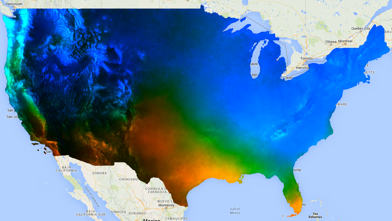
Figura 1: El resultado de linearFit() aplicado a la precipitación proyectada Las áreas en las que se prevé un aumento de las precipitaciones se muestran en azul y las que tendrán una disminución, en rojo.

linearRegression()

Por ejemplo, supongamos que hay dos variables dependientes: precipitación y temperatura máxima, y dos variables independientes: una constante y el tiempo. La recopilación es idéntica al ejemplo anterior, pero la banda constante se debe agregar de forma manual antes de la reducción. Las dos primeras bandas de la entrada son las variables “X” (independientes) y las siguientes dos bandas son las variables “Y” (dependientes). En este ejemplo, primero obtén los coeficientes de regresión y, luego, aplana la imagen del array para extraer las bandas de interés:

Editor de código (JavaScript)

// This function adds a time band to the image.
var createTimeBand = function(image) {
  // Scale milliseconds by a large constant.
  return image.addBands(image.metadata('system:time_start').divide(1e18));
};

// This function adds a constant band to the image.
var createConstantBand = function(image) {
  return ee.Image(1).addBands(image);
};

// Load the input image collection: projected climate data.
var collection = ee.ImageCollection('NASA/NEX-DCP30_ENSEMBLE_STATS')
  .filterDate(ee.Date('2006-01-01'), ee.Date('2099-01-01'))
  .filter(ee.Filter.eq('scenario', 'rcp85'))
  // Map the functions over the collection, to get constant and time bands.
  .map(createTimeBand)
  .map(createConstantBand)
  // Select the predictors and the responses.
  .select(['constant', 'system:time_start', 'pr_mean', 'tasmax_mean']);

// Compute ordinary least squares regression coefficients.
var linearRegression = collection.reduce(
  ee.Reducer.linearRegression({
    numX: 2,
    numY: 2
}));

// Compute robust linear regression coefficients.
var robustLinearRegression = collection.reduce(
  ee.Reducer.robustLinearRegression({
    numX: 2,
    numY: 2
}));

// The results are array images that must be flattened for display.
// These lists label the information along each axis of the arrays.
var bandNames = [['constant', 'time'], // 0-axis variation.
                 ['precip', 'temp']]; // 1-axis variation.

// Flatten the array images to get multi-band images according to the labels.
var lrImage = linearRegression.select(['coefficients']).arrayFlatten(bandNames);
var rlrImage = robustLinearRegression.select(['coefficients']).arrayFlatten(bandNames);

// Display the OLS results.
Map.setCenter(-100.11, 40.38, 5);
Map.addLayer(lrImage,
  {min: 0, max: [-0.9, 8e-5, 1], bands: ['time_precip', 'constant_precip', 'time_precip']}, 'OLS');

// Compare the results at a specific point:
print('OLS estimates:', lrImage.reduceRegion({
  reducer: ee.Reducer.first(),
  geometry: ee.Geometry.Point([-96.0, 41.0]),
  scale: 1000
}));

print('Robust estimates:', rlrImage.reduceRegion({
  reducer: ee.Reducer.first(),
  geometry: ee.Geometry.Point([-96.0, 41.0]),
  scale: 1000
}));

Inspecciona los resultados para descubrir que el resultado de linearRegression() es equivalente a los coeficientes estimados por el reductor linearFit(), aunque el resultado de linearRegression() también tiene coeficientes para la otra variable dependiente, tasmax_mean. Los coeficientes de regresión lineal robustos son diferentes de las estimaciones de OLS. En el ejemplo, se comparan los coeficientes de los diferentes métodos de regresión en un punto específico.

ee.Image

En el contexto de un objeto ee.Image, los reductores de regresión se pueden usar con reduceRegion o reduceRegions para realizar una regresión lineal en los píxeles de las regiones. En los siguientes ejemplos, se muestra cómo calcular los coeficientes de regresión entre las bandas de Landsat en un polígono arbitrario.

linearFit()

En la sección de la guía que describe los gráficos de datos del array, se muestra un diagrama de dispersión de la correlación entre las bandas SWIR1 y SWIR2 de Landsat 8. Aquí, se calculan los coeficientes de regresión lineal para esta relación. Se muestra un diccionario que contiene las propiedades 'offset' (intercepto en Y) y 'scale' (pendiente).

Editor de código (JavaScript)

// Define a rectangle geometry around San Francisco.
var sanFrancisco = ee.Geometry.Rectangle([-122.45, 37.74, -122.4, 37.8]);

// Import a Landsat 8 TOA image for this region.
var img = ee.Image('LANDSAT/LC08/C02/T1_TOA/LC08_044034_20140318');

// Subset the SWIR1 and SWIR2 bands. In the regression reducer, independent
// variables come first followed by the dependent variables. In this case,
// B5 (SWIR1) is the independent variable and B6 (SWIR2) is the dependent
// variable.
var imgRegress = img.select(['B5', 'B6']);

// Calculate regression coefficients for the set of pixels intersecting the
// above defined region using reduceRegion with ee.Reducer.linearFit().
var linearFit = imgRegress.reduceRegion({
  reducer: ee.Reducer.linearFit(),
  geometry: sanFrancisco,
  scale: 30,
});

// Inspect the results.
print('OLS estimates:', linearFit);
print('y-intercept:', linearFit.get('offset'));
print('Slope:', linearFit.get('scale'));

linearRegression()

Aquí se aplica el mismo análisis de la sección linearFit anterior, excepto que esta vez se usa la función ee.Reducer.linearRegression. Ten en cuenta que una imagen de regresión se construye a partir de tres imágenes independientes: una imagen constante y las imágenes que representan las bandas SWIR1 y SWIR2 de la misma imagen de Landsat 8. Ten en cuenta que puedes combinar cualquier conjunto de bandas para construir una imagen de entrada para la reducción de regiones por ee.Reducer.linearRegression, no es necesario que pertenezcan a la misma imagen de origen.

Editor de código (JavaScript)

// Define a rectangle geometry around San Francisco.
var sanFrancisco = ee.Geometry.Rectangle([-122.45, 37.74, -122.4, 37.8]);

// Import a Landsat 8 TOA image for this region.
var img = ee.Image('LANDSAT/LC08/C02/T1_TOA/LC08_044034_20140318');

// Create a new image that is the concatenation of three images: a constant,
// the SWIR1 band, and the SWIR2 band.
var constant = ee.Image(1);
var xVar = img.select('B5');
var yVar = img.select('B6');
var imgRegress = ee.Image.cat(constant, xVar, yVar);

// Calculate regression coefficients for the set of pixels intersecting the
// above defined region using reduceRegion. The numX parameter is set as 2
// because the constant and the SWIR1 bands are independent variables and they
// are the first two bands in the stack; numY is set as 1 because there is only
// one dependent variable (SWIR2) and it follows as band three in the stack.
var linearRegression = imgRegress.reduceRegion({
  reducer: ee.Reducer.linearRegression({
    numX: 2,
    numY: 1
  }),
  geometry: sanFrancisco,
  scale: 30,
});

// Convert the coefficients array to a list.
var coefList = ee.Array(linearRegression.get('coefficients')).toList();

// Extract the y-intercept and slope.
var b0 = ee.List(coefList.get(0)).get(0); // y-intercept
var b1 = ee.List(coefList.get(1)).get(0); // slope

// Extract the residuals.
var residuals = ee.Array(linearRegression.get('residuals')).toList().get(0);

// Inspect the results.
print('OLS estimates', linearRegression);
print('y-intercept:', b0);
print('Slope:', b1);
print('Residuals:', residuals);

Se muestra un diccionario que contiene las propiedades 'coefficients' y 'residuals'. La propiedad 'coefficients' es un array con dimensiones (numX, numY); cada columna contiene los coeficientes de la variable dependiente correspondiente. En este caso, el array tiene dos filas y una columna. La fila uno, columna uno es la intersección y la fila dos, columna uno es la pendiente. La propiedad 'residuals' es el vector de la raíz cuadrada media de los residuos de cada variable dependiente. Para extraer los coeficientes, asigna el resultado como un array y, luego, corta los elementos deseados o convierte el array en una lista y selecciona los coeficientes por posición de índice.

ee.FeatureCollection

Supongamos que quieres conocer la relación lineal entre la reflectancia SWIR1 de Sentinel-2 y la de Landsat 8. En este ejemplo, se usa una muestra aleatoria de píxeles con formato de colección de componentes de puntos para calcular la relación. Se genera un diagrama de dispersión de los pares de píxeles junto con la línea de mínimos cuadrados de mejor ajuste (Figura 2).

Editor de código (JavaScript)

// Import a Sentinel-2 TOA image.
var s2ImgSwir1 = ee.Image('COPERNICUS/S2/20191022T185429_20191022T185427_T10SEH');

// Import a Landsat 8 TOA image from 12 days earlier than the S2 image.
var l8ImgSwir1 = ee.Image('LANDSAT/LC08/C02/T1_TOA/LC08_044033_20191010');

// Get the intersection between the two images - the area of interest (aoi).
var aoi = s2ImgSwir1.geometry().intersection(l8ImgSwir1.geometry());

// Get a set of 1000 random points from within the aoi. A feature collection
// is returned.
var sample = ee.FeatureCollection.randomPoints({
  region: aoi,
  points: 1000
});

// Combine the SWIR1 bands from each image into a single image.
var swir1Bands = s2ImgSwir1.select('B11')
  .addBands(l8ImgSwir1.select('B6'))
  .rename(['s2_swir1', 'l8_swir1']);

// Sample the SWIR1 bands using the sample point feature collection.
var imgSamp = swir1Bands.sampleRegions({
  collection: sample,
  scale: 30
})
// Add a constant property to each feature to be used as an independent variable.
.map(function(feature) {
  return feature.set('constant', 1);
});

// Compute linear regression coefficients. numX is 2 because
// there are two independent variables: 'constant' and 's2_swir1'. numY is 1
// because there is a single dependent variable: 'l8_swir1'. Cast the resulting
// object to an ee.Dictionary for easy access to the properties.
var linearRegression = ee.Dictionary(imgSamp.reduceColumns({
  reducer: ee.Reducer.linearRegression({
    numX: 2,
    numY: 1
  }),
  selectors: ['constant', 's2_swir1', 'l8_swir1']
}));

// Convert the coefficients array to a list.
var coefList = ee.Array(linearRegression.get('coefficients')).toList();

// Extract the y-intercept and slope.
var yInt = ee.List(coefList.get(0)).get(0); // y-intercept
var slope = ee.List(coefList.get(1)).get(0); // slope

// Gather the SWIR1 values from the point sample into a list of lists.
var props = ee.List(['s2_swir1', 'l8_swir1']);
var regressionVarsList = ee.List(imgSamp.reduceColumns({
  reducer: ee.Reducer.toList().repeat(props.size()),
  selectors: props
}).get('list'));

// Convert regression x and y variable lists to an array - used later as input
// to ui.Chart.array.values for generating a scatter plot.
var x = ee.Array(ee.List(regressionVarsList.get(0)));
var y1 = ee.Array(ee.List(regressionVarsList.get(1)));

// Apply the line function defined by the slope and y-intercept of the
// regression to the x variable list to create an array that will represent
// the regression line in the scatter plot.
var y2 = ee.Array(ee.List(regressionVarsList.get(0)).map(function(x) {
  var y = ee.Number(x).multiply(slope).add(yInt);
  return y;
}));

// Concatenate the y variables (Landsat 8 SWIR1 and predicted y) into an array
// for input to ui.Chart.array.values for plotting a scatter plot.
var yArr = ee.Array.cat([y1, y2], 1);

// Make a scatter plot of the two SWIR1 bands for the point sample and include
// the least squares line of best fit through the data.
print(ui.Chart.array.values({
  array: yArr,
  axis: 0,
  xLabels: x})
  .setChartType('ScatterChart')
  .setOptions({
    legend: {position: 'none'},
    hAxis: {'title': 'Sentinel-2 SWIR1'},
    vAxis: {'title': 'Landsat 8 SWIR1'},
    series: {
      0: {
        pointSize: 0.2,
        dataOpacity: 0.5,
      },
      1: {
        pointSize: 0,
        lineWidth: 2,
      }
    }
  })
);

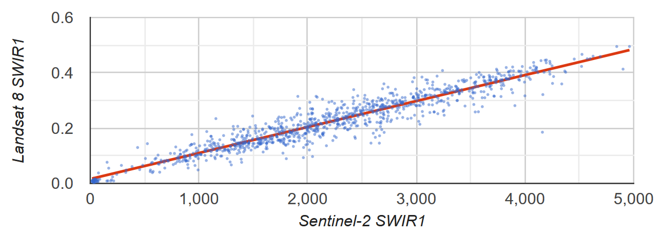
Figura 2: Gráfico de dispersión y línea de regresión lineal de mínimos cuadrados para una muestra de píxeles que representan la reflectancia de la TOA SWIR1 de Sentinel-2 y Landsat 8.

ee.List

Las columnas de objetos ee.List de 2D pueden ser entradas para los reductores de regresión. En los siguientes ejemplos, se proporcionan pruebas simples; la variable independiente es una copia de la variable dependiente que produce un eje Y interceptado igual a 0 y una pendiente igual a 1.

Nota: El resultado de la reducción de ee.List es un objeto. Transfórmala en un ee.Dictionary para facilitar el acceso a las propiedades.

Precaución: Las longitudes entre filas y columnas deben ser iguales. Usa null para representar las entradas de datos faltantes.

linearFit()

Editor de código (JavaScript)

// Define a list of lists, where columns represent variables. The first column
// is the independent variable and the second is the dependent variable.
var listsVarColumns = ee.List([
  [1, 1],
  [2, 2],
  [3, 3],
  [4, 4],
  [5, 5]
]);

// Compute the least squares estimate of a linear function. Note that an
// object is returned; cast it as an ee.Dictionary to make accessing the
// coefficients easier.
var linearFit = ee.Dictionary(listsVarColumns.reduce(ee.Reducer.linearFit()));

// Inspect the result.
print(linearFit);
print('y-intercept:', linearFit.get('offset'));
print('Slope:', linearFit.get('scale'));

Para transponer la lista si las variables están representadas por filas, conviértela en una ee.Array, transpósala y, luego, conviértela en una ee.List.

Editor de código (JavaScript)

// If variables in the list are arranged as rows, you'll need to transpose it.
// Define a list of lists where rows represent variables. The first row is the
// independent variable and the second is the dependent variable.
var listsVarRows = ee.List([
  [1, 2, 3, 4, 5],
  [1, 2, 3, 4, 5]
]);

// Cast the ee.List as an ee.Array, transpose it, and cast back to ee.List.
var listsVarColumns = ee.Array(listsVarRows).transpose().toList();

// Compute the least squares estimate of a linear function. Note that an
// object is returned; cast it as an ee.Dictionary to make accessing the
// coefficients easier.
var linearFit = ee.Dictionary(listsVarColumns.reduce(ee.Reducer.linearFit()));

// Inspect the result.
print(linearFit);
print('y-intercept:', linearFit.get('offset'));
print('Slope:', linearFit.get('scale'));

linearRegression()

La aplicación de ee.Reducer.linearRegression() es similar al ejemplo anterior de linearFit(), excepto que se incluye una variable independiente constante.

Editor de código (JavaScript)

// Define a list of lists where columns represent variables. The first column
// represents a constant term, the second an independent variable, and the third
// a dependent variable.
var listsVarColumns = ee.List([
  [1, 1, 1],
  [1, 2, 2],
  [1, 3, 3],
  [1, 4, 4],
  [1, 5, 5]
]);

// Compute ordinary least squares regression coefficients. numX is 2 because
// there is one constant term and an additional independent variable. numY is 1
// because there is only a single dependent variable. Cast the resulting
// object to an ee.Dictionary for easy access to the properties.
var linearRegression = ee.Dictionary(
  listsVarColumns.reduce(ee.Reducer.linearRegression({
    numX: 2,
    numY: 1
})));

// Convert the coefficients array to a list.
var coefList = ee.Array(linearRegression.get('coefficients')).toList();

// Extract the y-intercept and slope.
var b0 = ee.List(coefList.get(0)).get(0); // y-intercept
var b1 = ee.List(coefList.get(1)).get(0); // slope

// Extract the residuals.
var residuals = ee.Array(linearRegression.get('residuals')).toList().get(0);

// Inspect the results.
print('OLS estimates', linearRegression);
print('y-intercept:', b0);
print('Slope:', b1);
print('Residuals:', residuals);