Query POI counts by H3

The PLACES_COUNT_PER_H3 function aggregates Places of Interest (POI) data into standardized H3 spatial grid cells at a specified resolution. This function is the recommended pathway for regional density analysis, competitive mapping, and generating hexagonal choropleth heatmaps.

To call the PLACES_COUNT_PER_H3 function, use a SQL FROM clause because the function returns a table.

Syntax and parameters

SELECT * FROM `PROJECT_NAME.LINKED_DATASET_NAME.PLACES_COUNT_PER_H3`(
  filters
)

Parameters

• PROJECT_NAME: The name of your Google Cloud project. If you don't specify a project name, your query will default to the active project.
• LINKED_DATASET_NAME: The name of your subscribed Places Insights dataset (for example, places_insights___us).
• filters (JSON): A JSON object constructed using JSON_OBJECT containing key-value filter parameters.

Required JSON Filters

• geography (GEOGRAPHY): The bounding search area (Point, Linestring, or Polygon) to be indexed.
• h3_resolution (INTEGER): The H3 cell resolution level (supported values range from 0 to 11).

Optional JSON Filters

• Additional parameters such as types, business_status, price_level, and min_rating to filter the places counted within each cell. See the complete list of filter parameters.

Output table schema

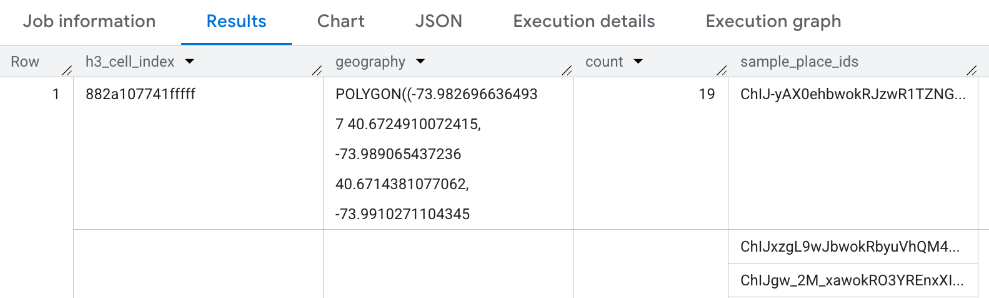
The function returns a BigQuery table with one row per H3 cell index intersecting your target geometry:

Column name	Data type	Description
h3_cell_index	STRING	The unique H3 index identifier for the cell.
geography	GEOGRAPHY	A polygon representing the physical boundary of the H3 cell.
count	INTEGER	The total exact count of matching operational places within this specific H3 cell, or zero if no places match.
sample_place_ids	ARRAY<STRING>	An array of up to 250 Place IDs located within this cell, enabling direct ground-truth queries using the Places API.

Aggregate regional POI density using PLACES_COUNT_PER_H3

The function processes the bounding geography specified in your filters, identifies all intersecting H3 hexagons at your target resolution, and returns exact place counts and Place IDs for each hexagon.

Example: Count wheelchair-accessible grocery and convenience stores in New York State

This query aggregates operational, wheelchair-accessible convenience and grocery stores in New York State using an H3 resolution level of 8. The boundary geometry of New York State is dynamically queried from the bigquery-public-data.geo_us_boundaries.states public dataset.

-- Query POI count per H3 cell intersecting the New York State polygon boundary
SELECT *
FROM `PROJECT_NAME.places_insights___us.PLACES_COUNT_PER_H3`(
  JSON_OBJECT(
      'geography', (
        -- Dynamically retrieve the boundary geography for New York State
        SELECT state_geom
        FROM `bigquery-public-data.geo_us_boundaries.states`
        WHERE state = 'NY'
        LIMIT 1
      ),
      'types', ['grocery_store', 'convenience_store'],
      'business_status', ['OPERATIONAL'],
      'h3_resolution', 8,
      'wheelchair_accessible_entrance', TRUE
  )
)
ORDER BY count DESC;

Response format

The query yields a row-by-row table mapping cells directly to spatial counts:

Important: The JSON object passed to PLACES_COUNT_PER_H3 is subject to a strict 1 MB size limit. Because the bounding geography is passed directly inside the JSON_OBJECT parameter under the 'geography' key, complex spatial boundaries with thousands of vertices can exceed this limit. To prevent execution failures, use the ST_SIMPLIFY function to reduce vertex complexity before passing geometries to the function.

Example: Count places per H3 cell filtered by brand

The following example uses the brand_ids filter to retrieve place counts and sample place IDs for specific brands, such as Starbucks "1413758728321880760" and Dunkin "1314981297593671295":

DECLARE geo GEOGRAPHY;

-- Get the geography for New York City.
SET geo = (SELECT geometry FROM `bigquery-public-data.overture_maps.division_area`
  WHERE country = 'US' AND subtype = 'locality' AND names.primary = 'New York'  LIMIT 1);

SELECT * FROM `PROJECT_NAME.places_insights___us.PLACES_COUNT_PER_H3`(
  JSON_OBJECT(
      'geography', geo,
      'h3_resolution', 8,
      'brand_ids', ["1413758728321880760", "1314981297593671295"],
      'business_status', ['OPERATIONAL']
    )
);

Visualize H3 results dynamically in Looker Studio

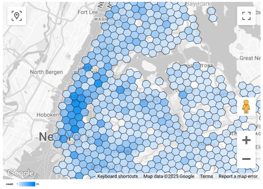
The following images show data from PLACES_COUNT_PER_H3 displayed in Looker Studio as a filled map. The darker the H3 cell, the higher the concentration of results:

To import your data into Looker Studio:

1. Run the function above in BigQuery to generate your results.
2. In the BigQuery results pane, click Open in -> Looker Studio. Your results are automatically imported into Looker Studio.

3. Looker Studio creates a default report page and initializes it with a title, table, and bar graph of the results.

   

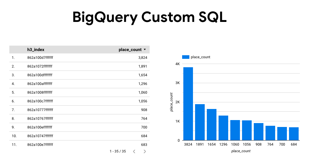
4. Select everything on the page and delete it.

5. Click Insert -> Filled map to add a filled map to your report.

6. Under Chart types -> Setup, configure the fields as shown below:

   

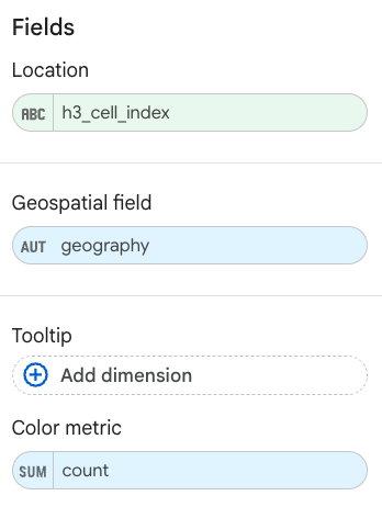
7. The filled map appears as above. You can optionally select Chart types -> Style to further configure the appearance of the map.

For more information on visualizing Places Insights results, see Visualize query results.