
以下のセクションでは、MIP の問題の例とその解決方法を説明します。これが問題です。
次の制約に従って x + 10y を最大化します。
x + 7y: 17.5 以下- 0 ~
x~ 3.5 - 0 ~
y x、y個の整数
制約は線形であるため、これは単なる線形最適化の問題であり、解は整数であることが必要です。以下のグラフは、問題に対する実行可能領域内の整数ポイントを示しています。
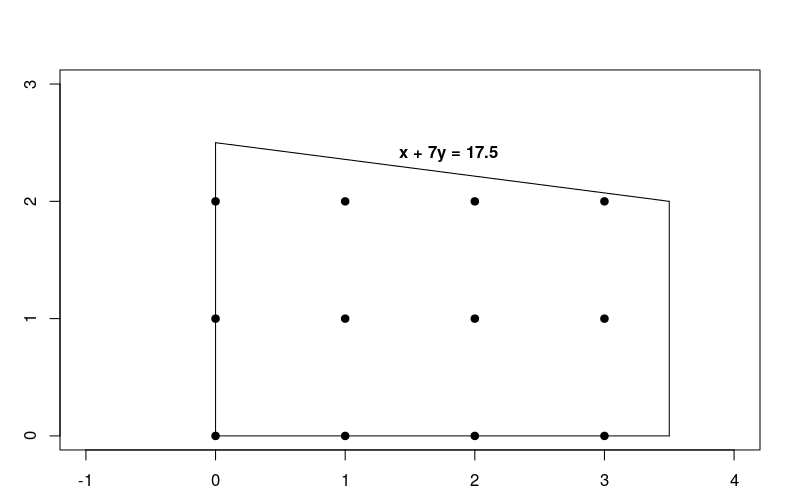
この問題は、LP 問題の解決で説明されている線形最適化の問題とよく似ていますが、解は整数でなければなりません。
MIP の問題を解決するための基本的な手順
MIP の問題を解決するには、プログラムに次のステップを含める必要があります。
- 線形ソルバーのラッパーをインポートします。
- MIP ソルバーを宣言する
- 変数を定義し、
- 制約を定義し、
- 目標を定義し
- MIP ソルバーを呼び出して、
- 解答を表示する
MPSolver を使用した解答
次のセクションでは、MPSolver ラッパーと MIP ソルバーを使用して問題を解決するプログラムを示します。
OR-Tools のデフォルトの MIP ソルバーは SCIP です。
線形ソルバーのラッパーをインポートする
以下に示すように、OR-Tools の線形ソルバー(MIP ソルバーと線形ソルバーのインターフェース)をインポートまたは追加します。
Python
from ortools.linear_solver import pywraplp
C++
#include <memory>

#include "ortools/linear_solver/linear_solver.h"
Java
import com.google.ortools.Loader;
import com.google.ortools.linearsolver.MPConstraint;
import com.google.ortools.linearsolver.MPObjective;
import com.google.ortools.linearsolver.MPSolver;
import com.google.ortools.linearsolver.MPVariable;
C#
using System;
using Google.OrTools.LinearSolver;
MIP ソルバーを宣言する
次のコードは問題の MIP ソルバーを宣言しています。この例では、サードパーティのソルバー SCIP を使用しています。
Python
# Create the mip solver with the SCIP backend.
solver = pywraplp.Solver.CreateSolver("SAT")
if not solver:
    return
C++
// Create the mip solver with the SCIP backend.
std::unique_ptr<MPSolver> solver(MPSolver::CreateSolver("SCIP"));
if (!solver) {
  LOG(WARNING) << "SCIP solver unavailable.";
  return;
}
Java
// Create the linear solver with the SCIP backend.
MPSolver solver = MPSolver.createSolver("SCIP");
if (solver == null) {
  System.out.println("Could not create solver SCIP");
  return;
}
C#
// Create the linear solver with the SCIP backend.
Solver solver = Solver.CreateSolver("SCIP");
if (solver is null)
{
    return;
}
変数を定義する
次のコードは、問題に含まれる変数を定義しています。
Python
infinity = solver.infinity()
# x and y are integer non-negative variables.
x = solver.IntVar(0.0, infinity, "x")
y = solver.IntVar(0.0, infinity, "y")

print("Number of variables =", solver.NumVariables())
C++
const double infinity = solver->infinity();
// x and y are integer non-negative variables.
MPVariable* const x = solver->MakeIntVar(0.0, infinity, "x");
MPVariable* const y = solver->MakeIntVar(0.0, infinity, "y");

LOG(INFO) << "Number of variables = " << solver->NumVariables();
Java
double infinity = java.lang.Double.POSITIVE_INFINITY;
// x and y are integer non-negative variables.
MPVariable x = solver.makeIntVar(0.0, infinity, "x");
MPVariable y = solver.makeIntVar(0.0, infinity, "y");

System.out.println("Number of variables = " + solver.numVariables());
C#
// x and y are integer non-negative variables.
Variable x = solver.MakeIntVar(0.0, double.PositiveInfinity, "x");
Variable y = solver.MakeIntVar(0.0, double.PositiveInfinity, "y");

Console.WriteLine("Number of variables = " + solver.NumVariables());
このプログラムは、MakeIntVar メソッド(コーディング言語によっては別のバリアント)を使用して、負でない整数値を受け取る変数 x と y を作成します。
制約を定義する
次のコードは、問題の制約を定義します。
Python
# x + 7 * y <= 17.5.
solver.Add(x + 7 * y <= 17.5)

# x <= 3.5.
solver.Add(x <= 3.5)

print("Number of constraints =", solver.NumConstraints())
C++
// x + 7 * y <= 17.5.
MPConstraint* const c0 = solver->MakeRowConstraint(-infinity, 17.5, "c0");
c0->SetCoefficient(x, 1);
c0->SetCoefficient(y, 7);

// x <= 3.5.
MPConstraint* const c1 = solver->MakeRowConstraint(-infinity, 3.5, "c1");
c1->SetCoefficient(x, 1);
c1->SetCoefficient(y, 0);

LOG(INFO) << "Number of constraints = " << solver->NumConstraints();
Java
// x + 7 * y <= 17.5.
MPConstraint c0 = solver.makeConstraint(-infinity, 17.5, "c0");
c0.setCoefficient(x, 1);
c0.setCoefficient(y, 7);

// x <= 3.5.
MPConstraint c1 = solver.makeConstraint(-infinity, 3.5, "c1");
c1.setCoefficient(x, 1);
c1.setCoefficient(y, 0);

System.out.println("Number of constraints = " + solver.numConstraints());
C#
// x + 7 * y <= 17.5.
solver.Add(x + 7 * y <= 17.5);

// x <= 3.5.
solver.Add(x <= 3.5);

Console.WriteLine("Number of constraints = " + solver.NumConstraints());
目標の設定
次のコードは、問題の objective function を定義しています。
Python
# Maximize x + 10 * y.
solver.Maximize(x + 10 * y)
C++
// Maximize x + 10 * y.
MPObjective* const objective = solver->MutableObjective();
objective->SetCoefficient(x, 1);
objective->SetCoefficient(y, 10);
objective->SetMaximization();
Java
// Maximize x + 10 * y.
MPObjective objective = solver.objective();
objective.setCoefficient(x, 1);
objective.setCoefficient(y, 10);
objective.setMaximization();
C#
// Maximize x + 10 * y.
solver.Maximize(x + 10 * y);
解法を呼び出す
次のコードはソルバーを呼び出します。
Python
print(f"Solving with {solver.SolverVersion()}")
status = solver.Solve()
C++
const MPSolver::ResultStatus result_status = solver->Solve();
// Check that the problem has an optimal solution.
if (result_status != MPSolver::OPTIMAL) {
  LOG(FATAL) << "The problem does not have an optimal solution!";
}
Java
final MPSolver.ResultStatus resultStatus = solver.solve();
C#
Solver.ResultStatus resultStatus = solver.Solve();
解答を表示する
次のコードは解答を示しています。
Python
if status == pywraplp.Solver.OPTIMAL:
    print("Solution:")
    print("Objective value =", solver.Objective().Value())
    print("x =", x.solution_value())
    print("y =", y.solution_value())
else:
    print("The problem does not have an optimal solution.")
C++
LOG(INFO) << "Solution:";
LOG(INFO) << "Objective value = " << objective->Value();
LOG(INFO) << "x = " << x->solution_value();
LOG(INFO) << "y = " << y->solution_value();
Java
if (resultStatus == MPSolver.ResultStatus.OPTIMAL) {
  System.out.println("Solution:");
  System.out.println("Objective value = " + objective.value());
  System.out.println("x = " + x.solutionValue());
  System.out.println("y = " + y.solutionValue());
} else {
  System.err.println("The problem does not have an optimal solution!");
}
C#
// Check that the problem has an optimal solution.
if (resultStatus != Solver.ResultStatus.OPTIMAL)
{
    Console.WriteLine("The problem does not have an optimal solution!");
    return;
}
Console.WriteLine("Solution:");
Console.WriteLine("Objective value = " + solver.Objective().Value());
Console.WriteLine("x = " + x.SolutionValue());
Console.WriteLine("y = " + y.SolutionValue());
問題の解決方法は次のとおりです。
Number of variables = 2
Number of constraints = 2
Solution:
Objective value = 23
x = 3
y = 2
目的関数の最適値は 23 で、これは点 x = 3、y = 2 で発生するものです。
プログラムを完了する
全プログラムは以下のとおりです。
Python
from ortools.linear_solver import pywraplp


def main():
    # Create the mip solver with the SCIP backend.
    solver = pywraplp.Solver.CreateSolver("SAT")
    if not solver:
        return

    infinity = solver.infinity()
    # x and y are integer non-negative variables.
    x = solver.IntVar(0.0, infinity, "x")
    y = solver.IntVar(0.0, infinity, "y")

    print("Number of variables =", solver.NumVariables())

    # x + 7 * y <= 17.5.
    solver.Add(x + 7 * y <= 17.5)

    # x <= 3.5.
    solver.Add(x <= 3.5)

    print("Number of constraints =", solver.NumConstraints())

    # Maximize x + 10 * y.
    solver.Maximize(x + 10 * y)

    print(f"Solving with {solver.SolverVersion()}")
    status = solver.Solve()

    if status == pywraplp.Solver.OPTIMAL:
        print("Solution:")
        print("Objective value =", solver.Objective().Value())
        print("x =", x.solution_value())
        print("y =", y.solution_value())
    else:
        print("The problem does not have an optimal solution.")

    print("\nAdvanced usage:")
    print(f"Problem solved in {solver.wall_time():d} milliseconds")
    print(f"Problem solved in {solver.iterations():d} iterations")
    print(f"Problem solved in {solver.nodes():d} branch-and-bound nodes")


if __name__ == "__main__":
    main()
C++
#include <memory>

#include "ortools/linear_solver/linear_solver.h"

namespace operations_research {
void SimpleMipProgram() {
  // Create the mip solver with the SCIP backend.
  std::unique_ptr<MPSolver> solver(MPSolver::CreateSolver("SCIP"));
  if (!solver) {
    LOG(WARNING) << "SCIP solver unavailable.";
    return;
  }

  const double infinity = solver->infinity();
  // x and y are integer non-negative variables.
  MPVariable* const x = solver->MakeIntVar(0.0, infinity, "x");
  MPVariable* const y = solver->MakeIntVar(0.0, infinity, "y");

  LOG(INFO) << "Number of variables = " << solver->NumVariables();

  // x + 7 * y <= 17.5.
  MPConstraint* const c0 = solver->MakeRowConstraint(-infinity, 17.5, "c0");
  c0->SetCoefficient(x, 1);
  c0->SetCoefficient(y, 7);

  // x <= 3.5.
  MPConstraint* const c1 = solver->MakeRowConstraint(-infinity, 3.5, "c1");
  c1->SetCoefficient(x, 1);
  c1->SetCoefficient(y, 0);

  LOG(INFO) << "Number of constraints = " << solver->NumConstraints();

  // Maximize x + 10 * y.
  MPObjective* const objective = solver->MutableObjective();
  objective->SetCoefficient(x, 1);
  objective->SetCoefficient(y, 10);
  objective->SetMaximization();

  const MPSolver::ResultStatus result_status = solver->Solve();
  // Check that the problem has an optimal solution.
  if (result_status != MPSolver::OPTIMAL) {
    LOG(FATAL) << "The problem does not have an optimal solution!";
  }

  LOG(INFO) << "Solution:";
  LOG(INFO) << "Objective value = " << objective->Value();
  LOG(INFO) << "x = " << x->solution_value();
  LOG(INFO) << "y = " << y->solution_value();

  LOG(INFO) << "\nAdvanced usage:";
  LOG(INFO) << "Problem solved in " << solver->wall_time() << " milliseconds";
  LOG(INFO) << "Problem solved in " << solver->iterations() << " iterations";
  LOG(INFO) << "Problem solved in " << solver->nodes()
            << " branch-and-bound nodes";
}
}  // namespace operations_research

int main(int argc, char** argv) {
  operations_research::SimpleMipProgram();
  return EXIT_SUCCESS;
}
Java
package com.google.ortools.linearsolver.samples;
import com.google.ortools.Loader;
import com.google.ortools.linearsolver.MPConstraint;
import com.google.ortools.linearsolver.MPObjective;
import com.google.ortools.linearsolver.MPSolver;
import com.google.ortools.linearsolver.MPVariable;

/** Minimal Mixed Integer Programming example to showcase calling the solver. */
public final class SimpleMipProgram {
  public static void main(String[] args) {
    Loader.loadNativeLibraries();
    // Create the linear solver with the SCIP backend.
    MPSolver solver = MPSolver.createSolver("SCIP");
    if (solver == null) {
      System.out.println("Could not create solver SCIP");
      return;
    }

    double infinity = java.lang.Double.POSITIVE_INFINITY;
    // x and y are integer non-negative variables.
    MPVariable x = solver.makeIntVar(0.0, infinity, "x");
    MPVariable y = solver.makeIntVar(0.0, infinity, "y");

    System.out.println("Number of variables = " + solver.numVariables());

    // x + 7 * y <= 17.5.
    MPConstraint c0 = solver.makeConstraint(-infinity, 17.5, "c0");
    c0.setCoefficient(x, 1);
    c0.setCoefficient(y, 7);

    // x <= 3.5.
    MPConstraint c1 = solver.makeConstraint(-infinity, 3.5, "c1");
    c1.setCoefficient(x, 1);
    c1.setCoefficient(y, 0);

    System.out.println("Number of constraints = " + solver.numConstraints());

    // Maximize x + 10 * y.
    MPObjective objective = solver.objective();
    objective.setCoefficient(x, 1);
    objective.setCoefficient(y, 10);
    objective.setMaximization();

    final MPSolver.ResultStatus resultStatus = solver.solve();

    if (resultStatus == MPSolver.ResultStatus.OPTIMAL) {
      System.out.println("Solution:");
      System.out.println("Objective value = " + objective.value());
      System.out.println("x = " + x.solutionValue());
      System.out.println("y = " + y.solutionValue());
    } else {
      System.err.println("The problem does not have an optimal solution!");
    }

    System.out.println("\nAdvanced usage:");
    System.out.println("Problem solved in " + solver.wallTime() + " milliseconds");
    System.out.println("Problem solved in " + solver.iterations() + " iterations");
    System.out.println("Problem solved in " + solver.nodes() + " branch-and-bound nodes");
  }

  private SimpleMipProgram() {}
}
C#
using System;
using Google.OrTools.LinearSolver;

public class SimpleMipProgram
{
    static void Main()
    {
        // Create the linear solver with the SCIP backend.
        Solver solver = Solver.CreateSolver("SCIP");
        if (solver is null)
        {
            return;
        }

        // x and y are integer non-negative variables.
        Variable x = solver.MakeIntVar(0.0, double.PositiveInfinity, "x");
        Variable y = solver.MakeIntVar(0.0, double.PositiveInfinity, "y");

        Console.WriteLine("Number of variables = " + solver.NumVariables());

        // x + 7 * y <= 17.5.
        solver.Add(x + 7 * y <= 17.5);

        // x <= 3.5.
        solver.Add(x <= 3.5);

        Console.WriteLine("Number of constraints = " + solver.NumConstraints());

        // Maximize x + 10 * y.
        solver.Maximize(x + 10 * y);

        Solver.ResultStatus resultStatus = solver.Solve();

        // Check that the problem has an optimal solution.
        if (resultStatus != Solver.ResultStatus.OPTIMAL)
        {
            Console.WriteLine("The problem does not have an optimal solution!");
            return;
        }
        Console.WriteLine("Solution:");
        Console.WriteLine("Objective value = " + solver.Objective().Value());
        Console.WriteLine("x = " + x.SolutionValue());
        Console.WriteLine("y = " + y.SolutionValue());

        Console.WriteLine("\nAdvanced usage:");
        Console.WriteLine("Problem solved in " + solver.WallTime() + " milliseconds");
        Console.WriteLine("Problem solved in " + solver.Iterations() + " iterations");
        Console.WriteLine("Problem solved in " + solver.Nodes() + " branch-and-bound nodes");
    }
}
線形最適化と整数最適化の比較
上記の整数最適化の問題の解と、整数の制約を取り除いた線形最適化の問題の解を比較してみましょう。整数問題の解は、線形解に最も近い実行可能領域(つまり、点 x = 0、y = 2)内の整数点であると推測されるかもしれません。ただし、次に説明するように、これは違います。
前のセクションのプログラムを次のように変更することで、線形問題を解決できます。
- MIP ソルバーの置き換え
解を求める
Python
# Create the mip solver with the SCIP backend.
solver = pywraplp.Solver.CreateSolver("SAT")
if not solver:
    return
C++
// Create the mip solver with the SCIP backend.
std::unique_ptr<MPSolver> solver(MPSolver::CreateSolver("SCIP"));
if (!solver) {
  LOG(WARNING) << "SCIP solver unavailable.";
  return;
}
Java
// Create the linear solver with the SCIP backend.
MPSolver solver = MPSolver.createSolver("SCIP");
if (solver == null) {
  System.out.println("Could not create solver SCIP");
  return;
}
C#
// Create the linear solver with the SCIP backend. Solver solver = Solver.CreateSolver("SCIP"); if (solver is null) { return; }Python
# Create the linear solver with the GLOP backend.
solver = pywraplp.Solver.CreateSolver("GLOP")
if not solver:
    return
C++
// Create the linear solver with the GLOP backend.
std::unique_ptr<MPSolver> solver(MPSolver::CreateSolver("GLOP"));
Java
// Create the linear solver with the GLOP backend.
MPSolver solver = MPSolver.createSolver("GLOP");
if (solver == null) {
  System.out.println("Could not create solver SCIP");
  return;
}
C#
// Create the linear solver with the GLOP backend. Solver solver = Solver.CreateSolver("GLOP"); if (solver is null) { return; } - 整数変数を置換する
連続変数の場合
Python
infinity = solver.infinity()
# x and y are integer non-negative variables.
x = solver.IntVar(0.0, infinity, "x")
y = solver.IntVar(0.0, infinity, "y")

print("Number of variables =", solver.NumVariables())
C++
const double infinity = solver->infinity();
// x and y are integer non-negative variables.
MPVariable* const x = solver->MakeIntVar(0.0, infinity, "x");
MPVariable* const y = solver->MakeIntVar(0.0, infinity, "y");

LOG(INFO) << "Number of variables = " << solver->NumVariables();
Java
double infinity = java.lang.Double.POSITIVE_INFINITY;
// x and y are integer non-negative variables.
MPVariable x = solver.makeIntVar(0.0, infinity, "x");
MPVariable y = solver.makeIntVar(0.0, infinity, "y");

System.out.println("Number of variables = " + solver.numVariables());
C#
// x and y are integer non-negative variables. Variable x = solver.MakeIntVar(0.0, double.PositiveInfinity, "x"); Variable y = solver.MakeIntVar(0.0, double.PositiveInfinity, "y"); Console.WriteLine("Number of variables = " + solver.NumVariables());Python
infinity = solver.infinity()
# Create the variables x and y.
x = solver.NumVar(0.0, infinity, "x")
y = solver.NumVar(0.0, infinity, "y")

print("Number of variables =", solver.NumVariables())
C++
const double infinity = solver->infinity();
// Create the variables x and y.
MPVariable* const x = solver->MakeNumVar(0.0, infinity, "x");
MPVariable* const y = solver->MakeNumVar(0.0, infinity, "y");

LOG(INFO) << "Number of variables = " << solver->NumVariables();
Java
double infinity = java.lang.Double.POSITIVE_INFINITY;
// Create the variables x and y.
MPVariable x = solver.makeNumVar(0.0, infinity, "x");
MPVariable y = solver.makeNumVar(0.0, infinity, "y");

System.out.println("Number of variables = " + solver.numVariables());
C#
// Create the variables x and y.
Variable x = solver.MakeNumVar(0.0, double.PositiveInfinity, "x");
Variable y = solver.MakeNumVar(0.0, double.PositiveInfinity, "y");

Console.WriteLine("Number of variables = " + solver.NumVariables());
これらの変更を行ってプログラムを再度実行すると、次の出力が表示されます。
Number of variables = 2
Number of constraints = 2
Objective value = 25.000000
x = 0.000000
y = 2.500000
線形問題の解は、目的関数が 25 に等しい x = 0、y = 2.5 の時点で発生します。これは線形問題と整数問題の両方に対する解答を示すグラフです
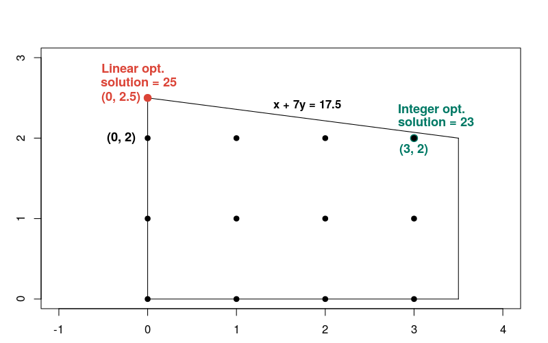
この整数解は、実行可能領域の他のほとんどの整数点と比べると、線形解には近くないことに注意してください。一般に、線形最適化の問題の解と、対応する整数の最適化の問題の解は、大きく異なります。このため、2 種類の問題の解決策には異なる方法が必要になります。