Esta página foi traduzida pela API Cloud Translation.

Resolução de problemas na página de destino

As seções a seguir apresentam um exemplo de problema de LP e mostram como resolvê-lo. Este é o problema:

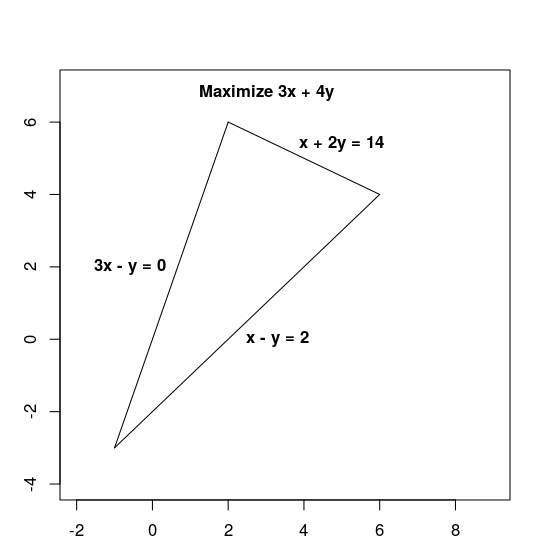
Maximize 3x + 4y sujeito às seguintes restrições:

x + 2y ≤ 14
3x - y ≥ 0
x - y ≤ 2

Tanto a função de objetivo, 3x + 4y quanto as restrições são fornecidas por expressões lineares, o que torna isso um problema linear.

As restrições definem a região viável, que é o triângulo mostrado abaixo, incluindo o interior dele.

Etapas básicas para resolver um problema de LP

Para resolver um problema de LP, o programa precisa incluir as seguintes etapas:

Importe o wrapper do solucionador linear
declarar o solucionador LP,
definir as variáveis,
definir as restrições,
definir o objetivo,
chame o solucionador LP e
mostrar a solução

Solução usando o MPSolver

Na seção a seguir, apresentamos um programa que resolve o problema usando o wrapper MPSolver e um solucionador LP.

Observação: Para executar o programa abaixo, você precisa instalar as ferramentas OR.

O solucionador principal de otimização linear das Ferramentas OR é o Glop, o solucionador de programação linear interno do Google. Ele é rápido, eficiente em termos de memória e numericamente estável.

Importar o wrapper do solucionador linear

Importe ou inclua o wrapper de solucionador linear OR-Tools, uma interface para solucionadores de MIP e solucionadores lineares, conforme mostrado abaixo.

Python

from ortools.linear_solver import pywraplp

C++

#include <iostream>
#include <memory>

#include "ortools/linear_solver/linear_solver.h"

Java

import com.google.ortools.Loader;
import com.google.ortools.linearsolver.MPConstraint;
import com.google.ortools.linearsolver.MPObjective;
import com.google.ortools.linearsolver.MPSolver;
import com.google.ortools.linearsolver.MPVariable;

C#

using System;
using Google.OrTools.LinearSolver;

Declarar o solucionador LP

MPsolver é um wrapper para vários solucionadores diferentes, incluindo o Glop. O código abaixo declara o solucionador GLOP.

Python

solver = pywraplp.Solver.CreateSolver("GLOP")
if not solver:
    return

C++

std::unique_ptr<MPSolver> solver(MPSolver::CreateSolver("SCIP"));
if (!solver) {
  LOG(WARNING) << "SCIP solver unavailable.";
  return;
}

Java

MPSolver solver = MPSolver.createSolver("GLOP");

C#

Solver solver = Solver.CreateSolver("GLOP");
if (solver is null)
{
    return;
}

Observação:substitua PDLP por GLOP para usar um solucionador de LP alternativo. Para mais detalhes sobre como escolher solucionadores, consulte Solução de LP avançada e, para instalar solucionadores de terceiros, consulte o guia de instalação.

Criar as variáveis

Primeiro, crie as variáveis x e y com valores que estão no intervalo de 0 a infinito.

Python

x = solver.NumVar(0, solver.infinity(), "x")
y = solver.NumVar(0, solver.infinity(), "y")

print("Number of variables =", solver.NumVariables())

C++

const double infinity = solver->infinity();
// x and y are non-negative variables.
MPVariable* const x = solver->MakeNumVar(0.0, infinity, "x");
MPVariable* const y = solver->MakeNumVar(0.0, infinity, "y");
LOG(INFO) << "Number of variables = " << solver->NumVariables();

Java

double infinity = java.lang.Double.POSITIVE_INFINITY;
// x and y are continuous non-negative variables.
MPVariable x = solver.makeNumVar(0.0, infinity, "x");
MPVariable y = solver.makeNumVar(0.0, infinity, "y");
System.out.println("Number of variables = " + solver.numVariables());

C#

Variable x = solver.MakeNumVar(0.0, double.PositiveInfinity, "x");
Variable y = solver.MakeNumVar(0.0, double.PositiveInfinity, "y");

Console.WriteLine("Number of variables = " + solver.NumVariables());

Definir as restrições

Em seguida, defina as restrições nas variáveis. Atribua um nome exclusivo a cada restrição (como constraint0) e defina os coeficientes da restrição.

Python

# Constraint 0: x + 2y <= 14.
solver.Add(x + 2 * y <= 14.0)

# Constraint 1: 3x - y >= 0.
solver.Add(3 * x - y >= 0.0)

# Constraint 2: x - y <= 2.
solver.Add(x - y <= 2.0)

print("Number of constraints =", solver.NumConstraints())

C++

// x + 2*y <= 14.
MPConstraint* const c0 = solver->MakeRowConstraint(-infinity, 14.0);
c0->SetCoefficient(x, 1);
c0->SetCoefficient(y, 2);

// 3*x - y >= 0.
MPConstraint* const c1 = solver->MakeRowConstraint(0.0, infinity);
c1->SetCoefficient(x, 3);
c1->SetCoefficient(y, -1);

// x - y <= 2.
MPConstraint* const c2 = solver->MakeRowConstraint(-infinity, 2.0);
c2->SetCoefficient(x, 1);
c2->SetCoefficient(y, -1);
LOG(INFO) << "Number of constraints = " << solver->NumConstraints();

Java

// x + 2*y <= 14.
MPConstraint c0 = solver.makeConstraint(-infinity, 14.0, "c0");
c0.setCoefficient(x, 1);
c0.setCoefficient(y, 2);

// 3*x - y >= 0.
MPConstraint c1 = solver.makeConstraint(0.0, infinity, "c1");
c1.setCoefficient(x, 3);
c1.setCoefficient(y, -1);

// x - y <= 2.
MPConstraint c2 = solver.makeConstraint(-infinity, 2.0, "c2");
c2.setCoefficient(x, 1);
c2.setCoefficient(y, -1);
System.out.println("Number of constraints = " + solver.numConstraints());

C#

// x + 2y <= 14.
solver.Add(x + 2 * y <= 14.0);

// 3x - y >= 0.
solver.Add(3 * x - y >= 0.0);

// x - y <= 2.
solver.Add(x - y <= 2.0);

Console.WriteLine("Number of constraints = " + solver.NumConstraints());

Definir a função objetiva

O código a seguir define a função de objetivo 3x + 4y e especifica que esse é um problema de maximização.

Python

# Objective function: 3x + 4y.
solver.Maximize(3 * x + 4 * y)

C++

// Objective function: 3x + 4y.
MPObjective* const objective = solver->MutableObjective();
objective->SetCoefficient(x, 3);
objective->SetCoefficient(y, 4);
objective->SetMaximization();

Java

// Maximize 3 * x + 4 * y.
MPObjective objective = solver.objective();
objective.setCoefficient(x, 3);
objective.setCoefficient(y, 4);
objective.setMaximization();

C#

// Objective function: 3x + 4y.
solver.Maximize(3 * x + 4 * y);

Invocar o solucionador

O código a seguir invoca o solucionador.

Python

print(f"Solving with {solver.SolverVersion()}")
status = solver.Solve()

C++

const MPSolver::ResultStatus result_status = solver->Solve();
// Check that the problem has an optimal solution.
if (result_status != MPSolver::OPTIMAL) {
  LOG(FATAL) << "The problem does not have an optimal solution!";
}

Java

final MPSolver.ResultStatus resultStatus = solver.solve();

C#

Solver.ResultStatus resultStatus = solver.Solve();

Mostrar a solução

O código a seguir exibe a solução.

Python

if status == pywraplp.Solver.OPTIMAL:
    print("Solution:")
    print(f"Objective value = {solver.Objective().Value():0.1f}")
    print(f"x = {x.solution_value():0.1f}")
    print(f"y = {y.solution_value():0.1f}")
else:
    print("The problem does not have an optimal solution.")

C++

LOG(INFO) << "Solution:";
LOG(INFO) << "Optimal objective value = " << objective->Value();
LOG(INFO) << x->name() << " = " << x->solution_value();
LOG(INFO) << y->name() << " = " << y->solution_value();

Java

if (resultStatus == MPSolver.ResultStatus.OPTIMAL) {
  System.out.println("Solution:");
  System.out.println("Objective value = " + objective.value());
  System.out.println("x = " + x.solutionValue());
  System.out.println("y = " + y.solutionValue());
} else {
  System.err.println("The problem does not have an optimal solution!");
}

C#

// Check that the problem has an optimal solution.
if (resultStatus != Solver.ResultStatus.OPTIMAL)
{
    Console.WriteLine("The problem does not have an optimal solution!");
    return;
}
Console.WriteLine("Solution:");
Console.WriteLine("Objective value = " + solver.Objective().Value());
Console.WriteLine("x = " + x.SolutionValue());
Console.WriteLine("y = " + y.SolutionValue());

Os programas completos

Os programas completos são mostrados abaixo.

Python

from ortools.linear_solver import pywraplp


def LinearProgrammingExample():
    """Linear programming sample."""
    # Instantiate a Glop solver, naming it LinearExample.
    solver = pywraplp.Solver.CreateSolver("GLOP")
    if not solver:
        return

    # Create the two variables and let them take on any non-negative value.
    x = solver.NumVar(0, solver.infinity(), "x")
    y = solver.NumVar(0, solver.infinity(), "y")

    print("Number of variables =", solver.NumVariables())

    # Constraint 0: x + 2y <= 14.
    solver.Add(x + 2 * y <= 14.0)

    # Constraint 1: 3x - y >= 0.
    solver.Add(3 * x - y >= 0.0)

    # Constraint 2: x - y <= 2.
    solver.Add(x - y <= 2.0)

    print("Number of constraints =", solver.NumConstraints())

    # Objective function: 3x + 4y.
    solver.Maximize(3 * x + 4 * y)

    # Solve the system.
    print(f"Solving with {solver.SolverVersion()}")
    status = solver.Solve()

    if status == pywraplp.Solver.OPTIMAL:
        print("Solution:")
        print(f"Objective value = {solver.Objective().Value():0.1f}")
        print(f"x = {x.solution_value():0.1f}")
        print(f"y = {y.solution_value():0.1f}")
    else:
        print("The problem does not have an optimal solution.")

    print("\nAdvanced usage:")
    print(f"Problem solved in {solver.wall_time():d} milliseconds")
    print(f"Problem solved in {solver.iterations():d} iterations")


LinearProgrammingExample()

C++

#include <iostream>
#include <memory>

#include "ortools/linear_solver/linear_solver.h"

namespace operations_research {
void LinearProgrammingExample() {
  std::unique_ptr<MPSolver> solver(MPSolver::CreateSolver("SCIP"));
  if (!solver) {
    LOG(WARNING) << "SCIP solver unavailable.";
    return;
  }

  const double infinity = solver->infinity();
  // x and y are non-negative variables.
  MPVariable* const x = solver->MakeNumVar(0.0, infinity, "x");
  MPVariable* const y = solver->MakeNumVar(0.0, infinity, "y");
  LOG(INFO) << "Number of variables = " << solver->NumVariables();

  // x + 2*y <= 14.
  MPConstraint* const c0 = solver->MakeRowConstraint(-infinity, 14.0);
  c0->SetCoefficient(x, 1);
  c0->SetCoefficient(y, 2);

  // 3*x - y >= 0.
  MPConstraint* const c1 = solver->MakeRowConstraint(0.0, infinity);
  c1->SetCoefficient(x, 3);
  c1->SetCoefficient(y, -1);

  // x - y <= 2.
  MPConstraint* const c2 = solver->MakeRowConstraint(-infinity, 2.0);
  c2->SetCoefficient(x, 1);
  c2->SetCoefficient(y, -1);
  LOG(INFO) << "Number of constraints = " << solver->NumConstraints();

  // Objective function: 3x + 4y.
  MPObjective* const objective = solver->MutableObjective();
  objective->SetCoefficient(x, 3);
  objective->SetCoefficient(y, 4);
  objective->SetMaximization();

  const MPSolver::ResultStatus result_status = solver->Solve();
  // Check that the problem has an optimal solution.
  if (result_status != MPSolver::OPTIMAL) {
    LOG(FATAL) << "The problem does not have an optimal solution!";
  }

  LOG(INFO) << "Solution:";
  LOG(INFO) << "Optimal objective value = " << objective->Value();
  LOG(INFO) << x->name() << " = " << x->solution_value();
  LOG(INFO) << y->name() << " = " << y->solution_value();
}
}  // namespace operations_research

int main(int argc, char** argv) {
  operations_research::LinearProgrammingExample();
  return EXIT_SUCCESS;
}

Java

package com.google.ortools.linearsolver.samples;
import com.google.ortools.Loader;
import com.google.ortools.linearsolver.MPConstraint;
import com.google.ortools.linearsolver.MPObjective;
import com.google.ortools.linearsolver.MPSolver;
import com.google.ortools.linearsolver.MPVariable;

/** Simple linear programming example. */
public final class LinearProgrammingExample {
  public static void main(String[] args) {
    Loader.loadNativeLibraries();
    MPSolver solver = MPSolver.createSolver("GLOP");

    double infinity = java.lang.Double.POSITIVE_INFINITY;
    // x and y are continuous non-negative variables.
    MPVariable x = solver.makeNumVar(0.0, infinity, "x");
    MPVariable y = solver.makeNumVar(0.0, infinity, "y");
    System.out.println("Number of variables = " + solver.numVariables());

    // x + 2*y <= 14.
    MPConstraint c0 = solver.makeConstraint(-infinity, 14.0, "c0");
    c0.setCoefficient(x, 1);
    c0.setCoefficient(y, 2);

    // 3*x - y >= 0.
    MPConstraint c1 = solver.makeConstraint(0.0, infinity, "c1");
    c1.setCoefficient(x, 3);
    c1.setCoefficient(y, -1);

    // x - y <= 2.
    MPConstraint c2 = solver.makeConstraint(-infinity, 2.0, "c2");
    c2.setCoefficient(x, 1);
    c2.setCoefficient(y, -1);
    System.out.println("Number of constraints = " + solver.numConstraints());

    // Maximize 3 * x + 4 * y.
    MPObjective objective = solver.objective();
    objective.setCoefficient(x, 3);
    objective.setCoefficient(y, 4);
    objective.setMaximization();

    final MPSolver.ResultStatus resultStatus = solver.solve();

    if (resultStatus == MPSolver.ResultStatus.OPTIMAL) {
      System.out.println("Solution:");
      System.out.println("Objective value = " + objective.value());
      System.out.println("x = " + x.solutionValue());
      System.out.println("y = " + y.solutionValue());
    } else {
      System.err.println("The problem does not have an optimal solution!");
    }

    System.out.println("\nAdvanced usage:");
    System.out.println("Problem solved in " + solver.wallTime() + " milliseconds");
    System.out.println("Problem solved in " + solver.iterations() + " iterations");
  }

  private LinearProgrammingExample() {}
}

C#

using System;
using Google.OrTools.LinearSolver;

public class LinearProgrammingExample
{
    static void Main()
    {
        Solver solver = Solver.CreateSolver("GLOP");
        if (solver is null)
        {
            return;
        }
        // x and y are continuous non-negative variables.
        Variable x = solver.MakeNumVar(0.0, double.PositiveInfinity, "x");
        Variable y = solver.MakeNumVar(0.0, double.PositiveInfinity, "y");

        Console.WriteLine("Number of variables = " + solver.NumVariables());

        // x + 2y <= 14.
        solver.Add(x + 2 * y <= 14.0);

        // 3x - y >= 0.
        solver.Add(3 * x - y >= 0.0);

        // x - y <= 2.
        solver.Add(x - y <= 2.0);

        Console.WriteLine("Number of constraints = " + solver.NumConstraints());

        // Objective function: 3x + 4y.
        solver.Maximize(3 * x + 4 * y);

        Solver.ResultStatus resultStatus = solver.Solve();

        // Check that the problem has an optimal solution.
        if (resultStatus != Solver.ResultStatus.OPTIMAL)
        {
            Console.WriteLine("The problem does not have an optimal solution!");
            return;
        }
        Console.WriteLine("Solution:");
        Console.WriteLine("Objective value = " + solver.Objective().Value());
        Console.WriteLine("x = " + x.SolutionValue());
        Console.WriteLine("y = " + y.SolutionValue());

        Console.WriteLine("\nAdvanced usage:");
        Console.WriteLine("Problem solved in " + solver.WallTime() + " milliseconds");
        Console.WriteLine("Problem solved in " + solver.Iterations() + " iterations");
    }
}

Solução ideal

O programa retorna a solução ideal para o problema, conforme mostrado abaixo.

Number of variables = 2
Number of constraints = 3
Solution:
x = 6.0
y = 4.0
Optimal objective value = 34.0

Confira um gráfico que mostra a solução:

A linha verde tracejada é definida ao definir a função de objetivo igual ao valor ideal de 34. Qualquer linha cuja equação tenha a forma 3x + 4y = c é paralela à linha tracejada, e 34 é o maior valor de c para o qual a linha cruza a região viável.

Para saber mais sobre como resolver problemas de otimização linear, consulte Solução de LP avançada.

Resolução de problemas na página de destino Mantenha tudo organizado com as coleções Salve e categorize o conteúdo com base nas suas preferências.

Etapas básicas para resolver um problema de LP

Solução usando o MPSolver

Importar o wrapper do solucionador linear

Python

C++

Java

C#

Declarar o solucionador LP

Python

C++

Java

C#

Criar as variáveis

Python

C++

Java

C#

Definir as restrições

Python

C++

Java

C#

Definir a função objetiva

Python

C++

Java

C#

Invocar o solucionador

Python

C++

Java

C#

Mostrar a solução

Python

C++

Java

C#

Os programas completos

Python

C++

Java

C#

Solução ideal

Resolução de problemas na página de destino