
Les sections suivantes présentent un exemple de problème LP et montrent comment le résoudre. Voici le problème:
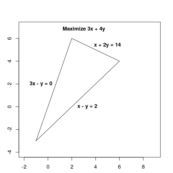
Maximisez la 3x + 4y sous réserve des contraintes suivantes:
x + 2y≤ 143x - y≥ 0x - y≤ 2
La fonction objectif 3x + 4y et les contraintes sont données par des expressions linéaires, ce qui en fait un problème linéaire.
Les contraintes définissent la région réalisable, c'est-à-dire le triangle ci-dessous, y compris son intérieur.
Étapes de base à suivre pour résoudre un problème lié à la page de destination
Pour résoudre un problème lié à la page de destination, votre programme doit inclure les étapes suivantes:
- Importer le wrapper de solution linéaire
- déclarer le résolveur LP,
- définir les variables,
- définir les contraintes,
- définir l'objectif,
- appeler le résolveur LP ; et
- afficher la solution
Solution utilisant le MPSolver
La section suivante présente un programme qui résout le problème à l'aide du wrapper MPSolver et d'un résolveur LP.
Remarque : Pour exécuter le programme ci-dessous, vous devez installer OR-Tools.
Le principal solution d'optimisation linéaire OR-Tools est Glop, le résolveur de programmation linéaire interne de Google. Il est rapide, efficace en termes de mémoire et stable numériquement.
Importer le wrapper de solution linéaire
Importez (ou incluez) le wrapper de solution linéaire OR-Tools, une interface pour les résolveurs MIP et les résolveurs linéaires, comme indiqué ci-dessous.
Python
from ortools.linear_solver import pywraplp
C++
#include <iostream>
#include <memory>

#include "ortools/linear_solver/linear_solver.h"
Java
import com.google.ortools.Loader;
import com.google.ortools.linearsolver.MPConstraint;
import com.google.ortools.linearsolver.MPObjective;
import com.google.ortools.linearsolver.MPSolver;
import com.google.ortools.linearsolver.MPVariable;
C#
using System;
using Google.OrTools.LinearSolver;
Déclarer le résolveur LP
MPsolver est un wrapper pour plusieurs résolveurs, y compris Glop. Le code ci-dessous déclare le résolveur GLOP.
Python
solver = pywraplp.Solver.CreateSolver("GLOP")
if not solver:
    return
C++
std::unique_ptr<MPSolver> solver(MPSolver::CreateSolver("SCIP"));
if (!solver) {
  LOG(WARNING) << "SCIP solver unavailable.";
  return;
}
Java
MPSolver solver = MPSolver.createSolver("GLOP");
C#
Solver solver = Solver.CreateSolver("GLOP");
if (solver is null)
{
    return;
}
Remarque:Remplacez PDLP par GLOP pour utiliser un autre outil de résolution de pages de destination. Pour en savoir plus sur le choix des résolveurs, consultez la page Résolution avancée de pages de destination. Pour l'installation de résolveurs tiers, consultez le guide d'installation.
Créer les variables
Commencez par créer les variables x et y dont les valeurs sont comprises entre 0 et l'infini.
Python
x = solver.NumVar(0, solver.infinity(), "x")
y = solver.NumVar(0, solver.infinity(), "y")

print("Number of variables =", solver.NumVariables())
C++
const double infinity = solver->infinity();
// x and y are non-negative variables.
MPVariable* const x = solver->MakeNumVar(0.0, infinity, "x");
MPVariable* const y = solver->MakeNumVar(0.0, infinity, "y");
LOG(INFO) << "Number of variables = " << solver->NumVariables();
Java
double infinity = java.lang.Double.POSITIVE_INFINITY;
// x and y are continuous non-negative variables.
MPVariable x = solver.makeNumVar(0.0, infinity, "x");
MPVariable y = solver.makeNumVar(0.0, infinity, "y");
System.out.println("Number of variables = " + solver.numVariables());
C#
Variable x = solver.MakeNumVar(0.0, double.PositiveInfinity, "x");
Variable y = solver.MakeNumVar(0.0, double.PositiveInfinity, "y");

Console.WriteLine("Number of variables = " + solver.NumVariables());
Définir les contraintes
Ensuite, définissez les contraintes sur les variables. Attribuez un nom unique à chaque contrainte (par exemple, constraint0), puis définissez les coefficients de la contrainte.
Python
# Constraint 0: x + 2y <= 14.
solver.Add(x + 2 * y <= 14.0)

# Constraint 1: 3x - y >= 0.
solver.Add(3 * x - y >= 0.0)

# Constraint 2: x - y <= 2.
solver.Add(x - y <= 2.0)

print("Number of constraints =", solver.NumConstraints())
C++
// x + 2*y <= 14.
MPConstraint* const c0 = solver->MakeRowConstraint(-infinity, 14.0);
c0->SetCoefficient(x, 1);
c0->SetCoefficient(y, 2);

// 3*x - y >= 0.
MPConstraint* const c1 = solver->MakeRowConstraint(0.0, infinity);
c1->SetCoefficient(x, 3);
c1->SetCoefficient(y, -1);

// x - y <= 2.
MPConstraint* const c2 = solver->MakeRowConstraint(-infinity, 2.0);
c2->SetCoefficient(x, 1);
c2->SetCoefficient(y, -1);
LOG(INFO) << "Number of constraints = " << solver->NumConstraints();
Java
// x + 2*y <= 14.
MPConstraint c0 = solver.makeConstraint(-infinity, 14.0, "c0");
c0.setCoefficient(x, 1);
c0.setCoefficient(y, 2);

// 3*x - y >= 0.
MPConstraint c1 = solver.makeConstraint(0.0, infinity, "c1");
c1.setCoefficient(x, 3);
c1.setCoefficient(y, -1);

// x - y <= 2.
MPConstraint c2 = solver.makeConstraint(-infinity, 2.0, "c2");
c2.setCoefficient(x, 1);
c2.setCoefficient(y, -1);
System.out.println("Number of constraints = " + solver.numConstraints());
C#
// x + 2y <= 14.
solver.Add(x + 2 * y <= 14.0);

// 3x - y >= 0.
solver.Add(3 * x - y >= 0.0);

// x - y <= 2.
solver.Add(x - y <= 2.0);

Console.WriteLine("Number of constraints = " + solver.NumConstraints());
Définir la fonction objectif
Le code suivant définit la fonction d'objectif 3x + 4y et spécifie qu'il s'agit d'un problème de maximisation.
Python
# Objective function: 3x + 4y.
solver.Maximize(3 * x + 4 * y)
C++
// Objective function: 3x + 4y.
MPObjective* const objective = solver->MutableObjective();
objective->SetCoefficient(x, 3);
objective->SetCoefficient(y, 4);
objective->SetMaximization();
Java
// Maximize 3 * x + 4 * y.
MPObjective objective = solver.objective();
objective.setCoefficient(x, 3);
objective.setCoefficient(y, 4);
objective.setMaximization();
C#
// Objective function: 3x + 4y.
solver.Maximize(3 * x + 4 * y);
Appeler le résolveur
Le code suivant appelle le résolveur.
Python
print(f"Solving with {solver.SolverVersion()}")
status = solver.Solve()
C++
const MPSolver::ResultStatus result_status = solver->Solve();
// Check that the problem has an optimal solution.
if (result_status != MPSolver::OPTIMAL) {
  LOG(FATAL) << "The problem does not have an optimal solution!";
}
Java
final MPSolver.ResultStatus resultStatus = solver.solve();
C#
Solver.ResultStatus resultStatus = solver.Solve();
Afficher la solution
Le code suivant affiche la solution.
Python
if status == pywraplp.Solver.OPTIMAL:
    print("Solution:")
    print(f"Objective value = {solver.Objective().Value():0.1f}")
    print(f"x = {x.solution_value():0.1f}")
    print(f"y = {y.solution_value():0.1f}")
else:
    print("The problem does not have an optimal solution.")
C++
LOG(INFO) << "Solution:";
LOG(INFO) << "Optimal objective value = " << objective->Value();
LOG(INFO) << x->name() << " = " << x->solution_value();
LOG(INFO) << y->name() << " = " << y->solution_value();
Java
if (resultStatus == MPSolver.ResultStatus.OPTIMAL) {
  System.out.println("Solution:");
  System.out.println("Objective value = " + objective.value());
  System.out.println("x = " + x.solutionValue());
  System.out.println("y = " + y.solutionValue());
} else {
  System.err.println("The problem does not have an optimal solution!");
}
C#
// Check that the problem has an optimal solution.
if (resultStatus != Solver.ResultStatus.OPTIMAL)
{
    Console.WriteLine("The problem does not have an optimal solution!");
    return;
}
Console.WriteLine("Solution:");
Console.WriteLine("Objective value = " + solver.Objective().Value());
Console.WriteLine("x = " + x.SolutionValue());
Console.WriteLine("y = " + y.SolutionValue());
Programmes complets
Les programmes complets sont présentés ci-dessous.
Python
from ortools.linear_solver import pywraplp


def LinearProgrammingExample():
    """Linear programming sample."""
    # Instantiate a Glop solver, naming it LinearExample.
    solver = pywraplp.Solver.CreateSolver("GLOP")
    if not solver:
        return

    # Create the two variables and let them take on any non-negative value.
    x = solver.NumVar(0, solver.infinity(), "x")
    y = solver.NumVar(0, solver.infinity(), "y")

    print("Number of variables =", solver.NumVariables())

    # Constraint 0: x + 2y <= 14.
    solver.Add(x + 2 * y <= 14.0)

    # Constraint 1: 3x - y >= 0.
    solver.Add(3 * x - y >= 0.0)

    # Constraint 2: x - y <= 2.
    solver.Add(x - y <= 2.0)

    print("Number of constraints =", solver.NumConstraints())

    # Objective function: 3x + 4y.
    solver.Maximize(3 * x + 4 * y)

    # Solve the system.
    print(f"Solving with {solver.SolverVersion()}")
    status = solver.Solve()

    if status == pywraplp.Solver.OPTIMAL:
        print("Solution:")
        print(f"Objective value = {solver.Objective().Value():0.1f}")
        print(f"x = {x.solution_value():0.1f}")
        print(f"y = {y.solution_value():0.1f}")
    else:
        print("The problem does not have an optimal solution.")

    print("\nAdvanced usage:")
    print(f"Problem solved in {solver.wall_time():d} milliseconds")
    print(f"Problem solved in {solver.iterations():d} iterations")


LinearProgrammingExample()
C++
#include <iostream>
#include <memory>

#include "ortools/linear_solver/linear_solver.h"

namespace operations_research {
void LinearProgrammingExample() {
  std::unique_ptr<MPSolver> solver(MPSolver::CreateSolver("SCIP"));
  if (!solver) {
    LOG(WARNING) << "SCIP solver unavailable.";
    return;
  }

  const double infinity = solver->infinity();
  // x and y are non-negative variables.
  MPVariable* const x = solver->MakeNumVar(0.0, infinity, "x");
  MPVariable* const y = solver->MakeNumVar(0.0, infinity, "y");
  LOG(INFO) << "Number of variables = " << solver->NumVariables();

  // x + 2*y <= 14.
  MPConstraint* const c0 = solver->MakeRowConstraint(-infinity, 14.0);
  c0->SetCoefficient(x, 1);
  c0->SetCoefficient(y, 2);

  // 3*x - y >= 0.
  MPConstraint* const c1 = solver->MakeRowConstraint(0.0, infinity);
  c1->SetCoefficient(x, 3);
  c1->SetCoefficient(y, -1);

  // x - y <= 2.
  MPConstraint* const c2 = solver->MakeRowConstraint(-infinity, 2.0);
  c2->SetCoefficient(x, 1);
  c2->SetCoefficient(y, -1);
  LOG(INFO) << "Number of constraints = " << solver->NumConstraints();

  // Objective function: 3x + 4y.
  MPObjective* const objective = solver->MutableObjective();
  objective->SetCoefficient(x, 3);
  objective->SetCoefficient(y, 4);
  objective->SetMaximization();

  const MPSolver::ResultStatus result_status = solver->Solve();
  // Check that the problem has an optimal solution.
  if (result_status != MPSolver::OPTIMAL) {
    LOG(FATAL) << "The problem does not have an optimal solution!";
  }

  LOG(INFO) << "Solution:";
  LOG(INFO) << "Optimal objective value = " << objective->Value();
  LOG(INFO) << x->name() << " = " << x->solution_value();
  LOG(INFO) << y->name() << " = " << y->solution_value();
}
}  // namespace operations_research

int main(int argc, char** argv) {
  operations_research::LinearProgrammingExample();
  return EXIT_SUCCESS;
}
Java
package com.google.ortools.linearsolver.samples;
import com.google.ortools.Loader;
import com.google.ortools.linearsolver.MPConstraint;
import com.google.ortools.linearsolver.MPObjective;
import com.google.ortools.linearsolver.MPSolver;
import com.google.ortools.linearsolver.MPVariable;

/** Simple linear programming example. */
public final class LinearProgrammingExample {
  public static void main(String[] args) {
    Loader.loadNativeLibraries();
    MPSolver solver = MPSolver.createSolver("GLOP");

    double infinity = java.lang.Double.POSITIVE_INFINITY;
    // x and y are continuous non-negative variables.
    MPVariable x = solver.makeNumVar(0.0, infinity, "x");
    MPVariable y = solver.makeNumVar(0.0, infinity, "y");
    System.out.println("Number of variables = " + solver.numVariables());

    // x + 2*y <= 14.
    MPConstraint c0 = solver.makeConstraint(-infinity, 14.0, "c0");
    c0.setCoefficient(x, 1);
    c0.setCoefficient(y, 2);

    // 3*x - y >= 0.
    MPConstraint c1 = solver.makeConstraint(0.0, infinity, "c1");
    c1.setCoefficient(x, 3);
    c1.setCoefficient(y, -1);

    // x - y <= 2.
    MPConstraint c2 = solver.makeConstraint(-infinity, 2.0, "c2");
    c2.setCoefficient(x, 1);
    c2.setCoefficient(y, -1);
    System.out.println("Number of constraints = " + solver.numConstraints());

    // Maximize 3 * x + 4 * y.
    MPObjective objective = solver.objective();
    objective.setCoefficient(x, 3);
    objective.setCoefficient(y, 4);
    objective.setMaximization();

    final MPSolver.ResultStatus resultStatus = solver.solve();

    if (resultStatus == MPSolver.ResultStatus.OPTIMAL) {
      System.out.println("Solution:");
      System.out.println("Objective value = " + objective.value());
      System.out.println("x = " + x.solutionValue());
      System.out.println("y = " + y.solutionValue());
    } else {
      System.err.println("The problem does not have an optimal solution!");
    }

    System.out.println("\nAdvanced usage:");
    System.out.println("Problem solved in " + solver.wallTime() + " milliseconds");
    System.out.println("Problem solved in " + solver.iterations() + " iterations");
  }

  private LinearProgrammingExample() {}
}
C#
using System;
using Google.OrTools.LinearSolver;

public class LinearProgrammingExample
{
    static void Main()
    {
        Solver solver = Solver.CreateSolver("GLOP");
        if (solver is null)
        {
            return;
        }
        // x and y are continuous non-negative variables.
        Variable x = solver.MakeNumVar(0.0, double.PositiveInfinity, "x");
        Variable y = solver.MakeNumVar(0.0, double.PositiveInfinity, "y");

        Console.WriteLine("Number of variables = " + solver.NumVariables());

        // x + 2y <= 14.
        solver.Add(x + 2 * y <= 14.0);

        // 3x - y >= 0.
        solver.Add(3 * x - y >= 0.0);

        // x - y <= 2.
        solver.Add(x - y <= 2.0);

        Console.WriteLine("Number of constraints = " + solver.NumConstraints());

        // Objective function: 3x + 4y.
        solver.Maximize(3 * x + 4 * y);

        Solver.ResultStatus resultStatus = solver.Solve();

        // Check that the problem has an optimal solution.
        if (resultStatus != Solver.ResultStatus.OPTIMAL)
        {
            Console.WriteLine("The problem does not have an optimal solution!");
            return;
        }
        Console.WriteLine("Solution:");
        Console.WriteLine("Objective value = " + solver.Objective().Value());
        Console.WriteLine("x = " + x.SolutionValue());
        Console.WriteLine("y = " + y.SolutionValue());

        Console.WriteLine("\nAdvanced usage:");
        Console.WriteLine("Problem solved in " + solver.WallTime() + " milliseconds");
        Console.WriteLine("Problem solved in " + solver.Iterations() + " iterations");
    }
}
Solution optimale
Le programme renvoie la solution optimale au problème, comme indiqué ci-dessous.
Number of variables = 2
Number of constraints = 3
Solution:
x = 6.0
y = 4.0
Optimal objective value = 34.0
Voici un graphique illustrant la solution:
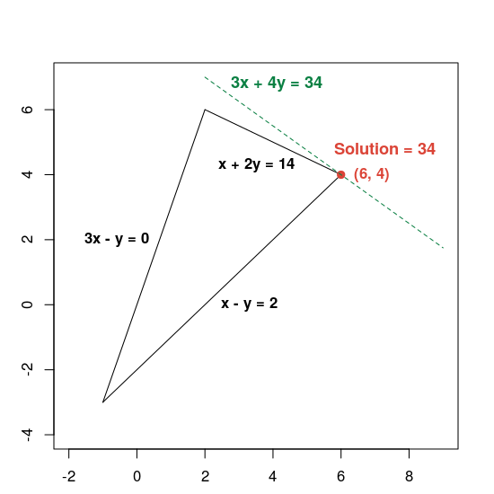
La ligne verte en pointillés est définie en définissant la fonction objectif sur sa valeur optimale (34). Toute ligne dont l'équation prend la forme 3x + 4y = c est parallèle à la ligne en pointillés, et 34 est la valeur de c la plus élevée pour laquelle la ligne croise la région réalisable.
Pour en savoir plus sur la résolution des problèmes d'optimisation linéaire, consultez la page Résolution avancée de la page de destination.