This section describes the default prior distributions for the Meridian
model. All prior distributions are specified by the prior_distribution
argument, which accepts a
PriorDistribution
object. Each parameter has its own argument in the PriorDistribution
constructor, and the joint prior distribution assumes that all of the priors are
independent.
Distributions can be specified as either a vector (such as,
tfp.distributions.Normal([1, 2, 3], [1, 1, 2])) or as a scalar (such as
tfp.distributions.Normal(1, 2)). All scalar distributions are broadcast to the
length of the parameter vector that they represent.
knot_values
Parameter: \(b_k\)
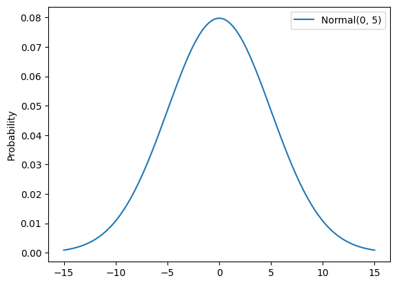
Default Prior: Normal(0, 5)
Rationale:
- Uninformative prior dictating how much time can have an effect.
- Uninformative because you want the flexibility to allow time to have a strong effect.
- Can be learned from the data given multiple geos per time period, and also multiple time periods per knot when the number of knots is low.
tau_g_excl_baseline
Parameter: \(\tau_g\)
Default Prior: Normal(0, 5)
Rationale:
- Uninformative prior dictating geo-differences.
- Uninformative because you want the flexibility to allow geo to have a strong effect.
- Can be learned from the data given multiple time periods per geo.
roi_m and roi_rf
Parameter: \(\text{ROI}_i^{[M]},\text{ROI}_{i}^{[RF]}\)
Default Prior: LogNormal(0.2, 0.9)
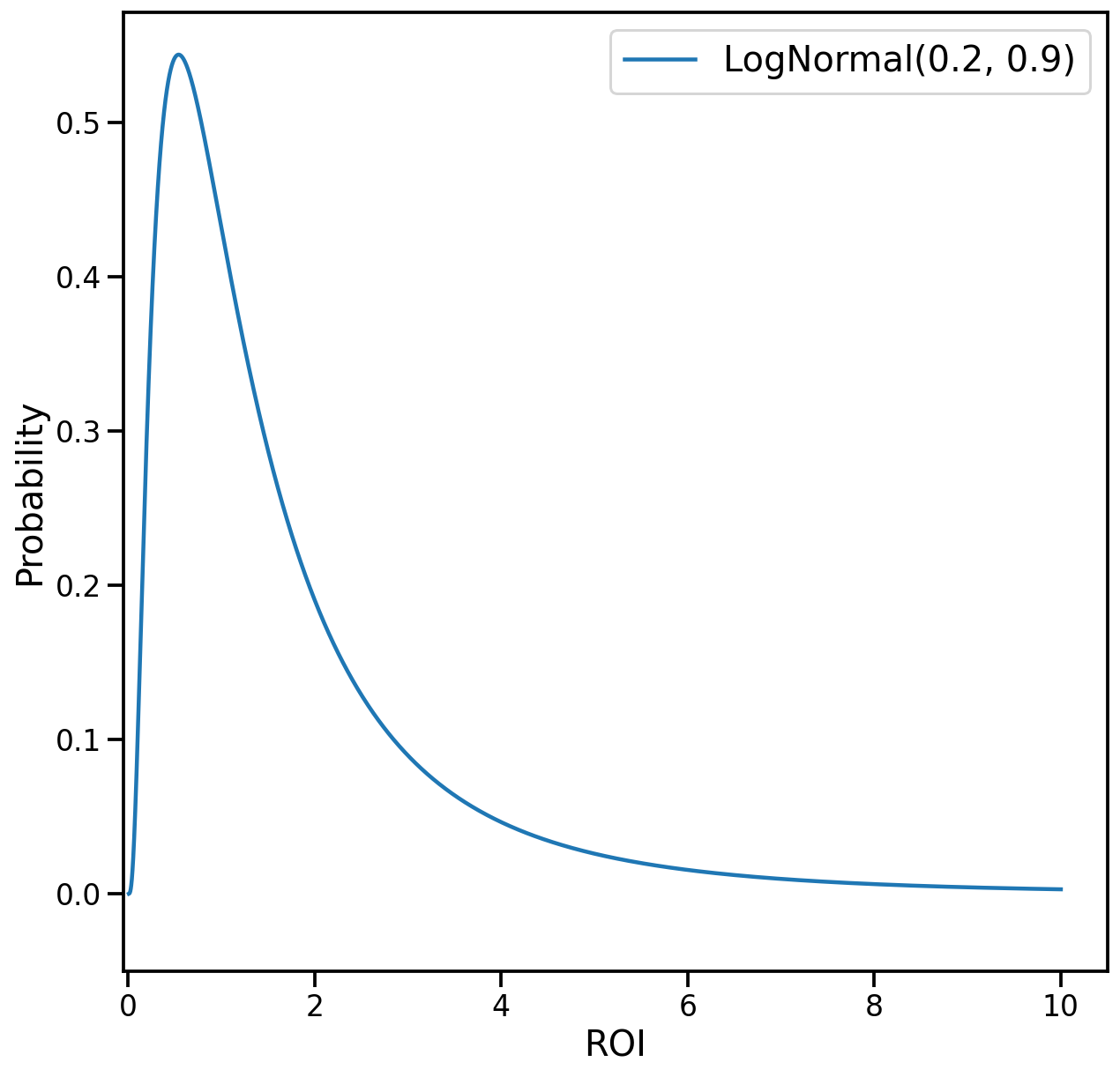
Rationale:
- This prior says that a priori the mean ROI of each channel is 1.83, 50% of ROIs are greater than 1.22, 80% are between 0.5 and 6.0, 95% are between 0.25 and 9.0, and 99% are less than 10.0.
- If the KPI is not revenue and revenue per KPI data is unavailable, a common ROI prior is placed on all channels such that the proportion of the KPI that is incremental due to all paid media channels has a prior mean of 40% and standard deviation of 20% (referred to as a "total paid media contribution prior"). For more considerations around this default, see Default total paid media contribution prior.
- The default distribution is strictly positive, which is required when media
coefficient random effects are log-normal
(
media_effects_dist='log_normal'). A prior allowing negative values could be used when random effects aremedia_effects_dist='normal', but this isn't generally recommended as it can inflate the posterior variance and cause MCMC sampling convergence problems.
mroi_m and mroi_rf
Parameter: \(\text{mROI}_i^{[M]},\text{mROI}_{i}^{[RF]}\)
Default Prior LogNormal(0.0, 0.5)

Rationale:
- This prior says that a priori the mean mROI of each channel is 1.13, 50% of mROIs are greater than 1.0, 80% are between 0.53 and 1.90, 95% are between 0.33 and 2.66, and 99% are less than 3.20.
- By default, each channel is assigned the same mROI prior.
- If the KPI is not revenue and revenue per KPI data is unavailable, mROI
priors can still be used, but you must specify a custom distribution for
roi_mandroi_rf. In this case, mROI is interpreted as incremental KPI units per spend unit (attributed to a small spend increase).
contribution_m, contribution_rf, contribution_om, and contribution_orf
Parameter: \(\text{Contribution}_i^{[M]},\text{Contribution}_{i}^{[RF]}\), \(\text{Contribution}_i^{[OM]},\text{Contribution}_{i}^{[ORF]}\)
Default Prior: Beta(1.0, 99.0)
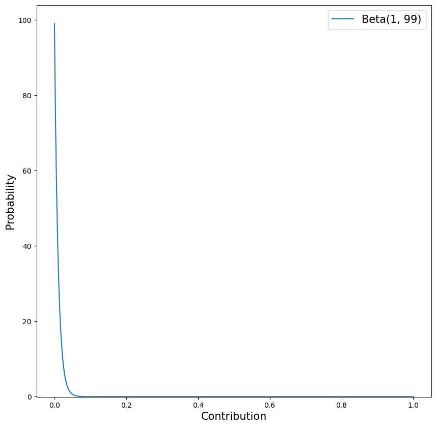
Rationale:
- The default prior says that a priori the mean contribution of each channel is 1%, 50% of contribution values are greater than 0.7%, 80% are between 0.1% and 2.3%, 95% are between 0.03% and 3.7%, and 99% are less than 4.5%.
- The default distribution does not allow the contribution of any individual channel to exceed 1.0 (100% of observed outcome). However, this does not necessarily prevent the combined contribution of multiple channels from exceeding 100%.
- The default distribution is strictly positive, which is required when media
coefficient random effects are log-normal
(
media_effects_dist='log_normal'). A prior allowing negative values could be used when random effects aremedia_effects_dist='normal', but this isn't generally recommended as it can inflate the posterior variance and cause MCMC sampling convergence problems. - The default distribution is fairly regularizing to mitigate MCMC convergence and negative baseline issues. Consider setting a custom prior that makes sense for your use case.
contribution_n
Parameter: \(\text{Contribution}_i^{[N]}\)
Default Prior: TruncatedNormal(0.0, 0.1, -1.0, 1.0)
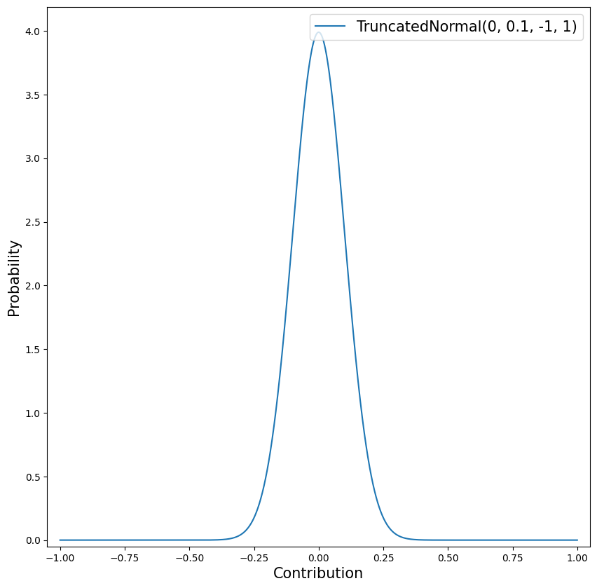
Rationale:
- The default prior says that a priori the mean and median contribution of each channel is 0% of total observed outcome, 80% are between -12.8% and +12.8%, and 95% are between -19.6% and +19.6%, and 99% are between -25.8% and +25.8%.
- The default prior allows negative values because non-media can have either a negative or positive contribution, depending on what the treatment is and what the corresponding baseline treatment value is. If you have prior knowledge that the contribution of a particular variable is strictly positive or negative, this should be incorporated into the prior.
beta_m, beta_rf, beta_om, and beta_orf
Parameter: \(\beta_i^{[M]},\beta_{i}^{[RF]},\beta_{i}^{[OM]}, \beta_{i}^{[ORF]}\)
Default Prior: HalfNormal(5)
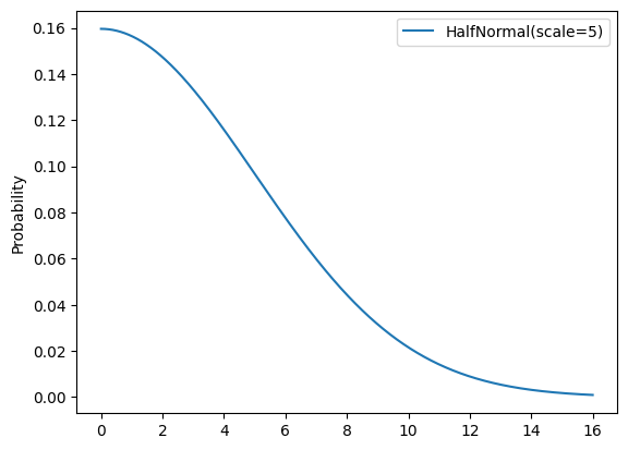
Rationale:
- Uninformative prior distribution on the parameter for the hierarchical
distribution of geo-level media effects for organic media channels for
impression and reach and frequency paid media channels respectively
(
beta_gom; beta_gorf). Whenmedia_effects_distis set to'normal', it is the hierarchical mean. Whenmedia_effects_distis set to'log_normal', it is the hierarchical parameter for the mean of the underlying, log-transformed,Normaldistribution. - Uninformative prior distribution on the parameter for the hierarchical
distribution of geo-level media effects for paid media channels for
impression and reach and frequency paid media channels respectively
(
beta_gm; beta_grf). Whenmedia_effects_distis set to'normal', it is the hierarchical mean. Whenmedia_effects_distis set to'log_normal', it is the hierarchical parameter for the mean of the underlying, log-transformed,Normaldistribution. - Uninformative because the interpretation of
beta_m,beta_rf,beta_omandbeta_orfcan vary widely given transformations, scaling, and the kind of media execution. - By default, Meridian uses ROI priors (
roi_mandroi_rf) for paid media channels. To usebeta_mandbeta_rfpriors for paid media, setmedia_prior_type='coefficient'andrf_prior_type='coefficient'. By default, Meridian uses contribution priors for organic media channels (
contribution_omandcontribution_orf). To usebeta_omandbeta_orfpriors for organic media, setorganic_media_prior_type='coefficient'andorganic_rf_prior_type='coefficient'.[M]denotes a paid media channel with impressions.[RF]denotes a paid media channel with reach and frequency.[OM]denotes an organic media channel with impressions.[ORF]denotes an organic media channel with reach and frequency.
eta_m, eta_rf, eta_om, and eta_orf
Parameter: \(\eta_i^{[M]},\eta_{i}^{[RF]},\eta_{i}^{[OM]}, \eta_{i}^{[ORF]}\)
Default Prior: HalfNormal(1)
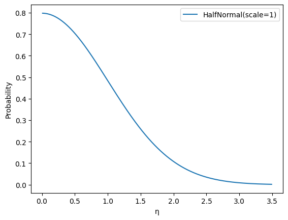
Rationale:
Moderate regularization encourages pooling across geos. This leads to lower variance estimates at the cost of increased bias, and allows the model to use the data more efficiently.
gamma_c and gamma_n
Parameter: \(\gamma_i^{[C]},\gamma_i^{[N]}\)
Default Prior: Normal(0, 5)
Rationale:
- Uninformative because of the wide range of control or non-media treatment variables you can possibly see.
- By default, Meridian uses contribution priors (
contribution_n) for non-media treatment channels. To usegamma_npriors for non-media treatments, setnon_media_treatments_prior_type='coefficient'.
xi_c and xi_n
Parameter: \(\xi_i^{[C]},\xi_i^{[N]}\)
Default Prior: HalfNormal(5)
Rationale:
- Uninformative to allow a wide range of geo variation in control and non-media treatment variable effects.
- By default, pooling is weaker for control and non-media treatment effects than for media effects because control effects are simple linear effects (without the complexity of Hill and Adstock transformations).
alpha_m, alpha_rf, alpha_om, and alpha_orf
Parameter: \(\alpha_i^{[M]},\alpha_{i}^{[RF]},\alpha_{i}^{[OM]}, \alpha_{i}^{[ORF]}\)
Default Prior: Uniform(0, 1)

Rationale:
Uninformative to allow data to inform the decay rate.
If you have intuition about the decay rate, consider setting a custom prior that makes sense for your use case. See The alpha prior for guidance on setting a custom prior.
ec_m and ec_om
Parameter: \(ec_i^{[M]}, ec_{i}^{[OM]}\)
Default Prior: TruncatedNormal(0.8, 0.8, 0.1, 10). This is the conditional
distribution \(X|0.1 < X < 10\), where \(X \sim N(0.8,0.8)\).
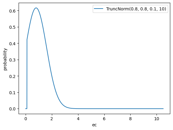
Rationale:
- The data is scaled such that when \(ec=1\), the half-saturation happens at the median of the non-zero media units per capita across geos and time. \(ec=X\) means that the half-saturation happens at \(X\) times the median of the non-zero media units per capita across geos and time.
- This prior has mean near one, which is a reasonable a priori assumption of where the half-saturation happens.
- The truncation is done to keep the parameter within a reasonable range for parameter identifiability.
- If a channel is way under-saturated (\(ec > 10\)) or way over-saturated
(\(ec < 0.1\)), the data does not really contain information about the
half-saturation point anyway. In such cases, the
ec_mparameter determines the shape of the response curve, but shouldn't be interpreted as an accurate estimate of half-saturation.
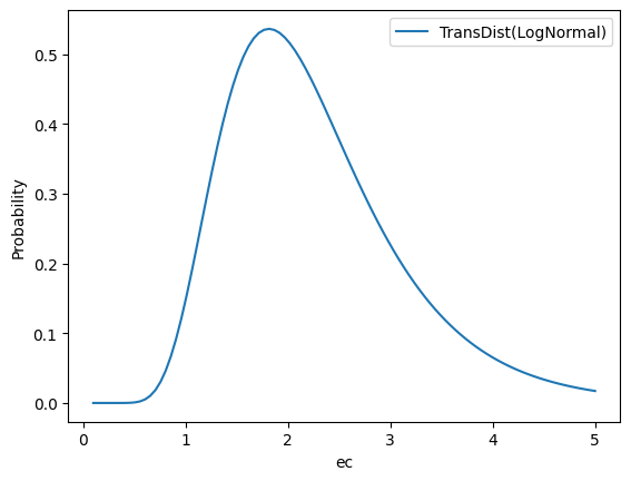
ec_rf and ec_orf
Parameter: \(ec_{i}^{[RF]},ec_{i}^{[ORF]}\)
Default Prior: LogNormal(0.7, 0.4) + 1
# Tensorflow Probability Syntax
tfp.distributions.TransformedDistribution(
    tfp.distributions.LogNormal(0.7, 0.4),
    tfp.bijectors.Shift(0.1)
)
Rationale:
- Moderately informative to prevent non-identification with
slope_rf. - Set in conjunction with the
slope_rfprior so that the prior distribution for optimal frequency has a mean of 2.1 and 90% CI of[1.0, 4.4]. This is considered to be a reasonable range of optimal frequency.
slope_m and slope_om
Parameter: \(\text{slope}_i^{[M]},\text{slope}_{i}^{[OM]}\)
Default Prior: Deterministic(1)
Rationale:
- Difficult to learn because of identifiability reasons.
Deterministic(1)means it is restricted to concave Hill curves.- The budget optimization algorithm produces a global optimum when Hill curves are concave. Changing this prior can lead to non-concave Hill curves and budget optimization can no longer produce a global optimum.
slope_rf and slope_orf
Parameter: \(\text{slope}_{i}^{[RF]},\text{slope}_{i}^{[ORF]}\)
Default Prior: LogNormal(0.7, 0.4)
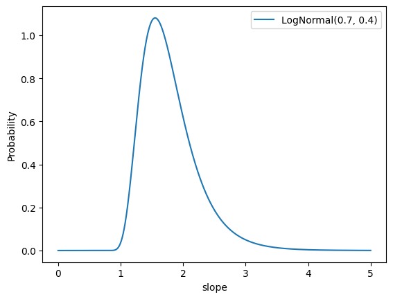
Rationale:
- Moderately informative to prevent non-identification with
ec_rf. Set in conjunction with the
ec_rfprior so that the prior distribution for optimal frequency has a mean of 2.1 and 90% CI of[1, 4.4], a reasonable range of optimal frequency.[M]denotes a paid media channel with impressions.[RF]denotes a paid media channel with reach and frequency.[OM]denotes an organic media channel with impressions.[ORF]denotes an organic media channel with reach and frequency.
sigma
Parameter: \(\sigma_g\)
Default Prior: HalfNormal(5)
Rationale:
Uninformative because residual variance varies widely by advertiser.