Page Summary
-
This guide presents a structured approach to hyperparameter tuning in machine learning, emphasizing the categorization of hyperparameters and deliberate experiment design.
-
The tuning process involves identifying scientific, nuisance, and fixed hyperparameters to efficiently explore the search space and optimize model performance.
-
Researchers should analyze training curves, isolate the impact of key hyperparameters, and carefully evaluate candidate changes for consistent improvements.
-
Automation is recommended for generating insightful plots and managing experiment results, while Bayesian optimization tools can be leveraged for final tuning.
-
Addressing issues like overfitting and step-to-step variance is crucial for achieving reliable and reproducible results in machine learning experiments.
For the purposes of this document:
The ultimate goal of machine learning development is to maximize the usefulness of the deployed model.
You can typically use the same basic steps and principles in this section on any ML problem.
This section makes the following assumptions:
- You already have a fully-running training pipeline along with a configuration that obtains a reasonable result.
- You have enough computational resources to conduct meaningful tuning experiments and to run at least several training jobs in parallel.
The incremental tuning strategy
Recommendation: Start with a simple configuration. Then, incrementally make improvements while building up insight into the problem. Make sure that any improvement is based on strong evidence.
We assume that your goal is to find a configuration that maximizes the performance of your model. Sometimes, your goal is to maximize model improvement by a fixed deadline. In other cases, you can keep improving the model indefinitely; for example, continually improving a model used in production.
In principle, you could maximize performance by using an algorithm to automatically search the entire space of possible configurations, but this is not a practical option. The space of possible configurations is extremely large and there are not yet any algorithms sophisticated enough to efficiently search this space without human guidance. Most automated search algorithms rely on a hand-designed search space that defines the set of configurations to search in, and these search spaces can matter quite a bit.
The most effective way to maximize performance is to start with a simple configuration and incrementally add features and make improvements while building up insight into the problem.
We recommend using automated search algorithms in each round of tuning and continually updating search spaces as your understanding grows. As you explore, you will naturally find better and better configurations and therefore your "best" model will continually improve.
The term "launch" refers to an update to our best configuration (which may or may not correspond to an actual launch of a production model). For each "launch," you must ensure that the change is based on strong evidence—not just random chance based on a lucky configuration—so that you don't add unnecessary complexity to the training pipeline.
At a high level, our incremental tuning strategy involves repeating the following four steps:
- Pick a goal for the next round of experiments. Make sure that the goal is appropriately scoped.
- Design the next round of experiments. Design and execute a set of experiments that progresses towards this goal.
- Learn from the experimental results. Evaluate the experiment against a checklist.
- Determine whether to adopt the candidate change.
The remainder of this section details this strategy.
Pick a goal for the next round of experiments
If you try to add multiple features or answer multiple questions at once, you may not be able to disentangle the separate effects on the results. Example goals include:
- Try a potential improvement to the pipeline (for example, a new regularizer, preprocessing choice, etc.).
- Understand the impact of a particular model hyperparameter (for example, the activation function)
- Minimize validation error.
Prioritize long term progress over short term validation error improvements
Summary: Most of the time, your primary goal is to gain insight into the tuning problem.
We recommend spending the majority of your time gaining insight into the problem and comparatively little time greedily focused on maximizing performance on the validation set. In other words, spend most of your time on "exploration" and only a small amount on "exploitation". Understanding the problem is critical to maximize final performance. Prioritizing insight over short term gains helps to:
- Avoid launching unnecessary changes that happened to be present in well-performing runs merely through historical accident.
- Identify which hyperparameters the validation error is most sensitive to, which hyperparameters interact the most and therefore need to be retuned together, and which hyperparameters are relatively insensitive to other changes and can therefore be fixed in future experiments.
- Suggest potential new features to try, such as new regularizers when overfitting is an issue.
- Identify features that don't help and therefore can be removed, reducing the complexity of future experiments.
- Recognize when improvements from hyperparameter tuning have likely saturated.
- Narrow our search spaces around the optimal value to improve tuning efficiency.
Eventually, you'll understand the problem. Then, you can focus purely on the validation error even if the experiments aren't maximally informative about the structure of the tuning problem.
Design the next round of experiments
Summary: Identify which hyperparameters are scientific, nuisance, and fixed hyperparameters for the experimental goal. Create a sequence of studies to compare different values of the scientific hyperparameters while optimizing over the nuisance hyperparameters. Choose the search space of nuisance hyperparameters to balance resource costs with scientific value.
Identify scientific, nuisance, and fixed hyperparameters
For a given goal, all hyperparameters fall into one of the following categories:
- scientific hyperparameters are those whose effect on the model's performance is what you're trying to measure.
- nuisance hyperparameters are those that need to be optimized over in order to fairly compare different values of the scientific hyperparameters. Nuisance hyperparameters are similar to nuisance parameters in statistics.
- fixed hyperparameters have constant values in the current round of experiments. The values of fixed hyperparameters shouldn't change when you compare different values of scientific hyperparameters. By fixing certain hyperparameters for a set of experiments, you must accept that conclusions derived from the experiments might not be valid for other settings of the fixed hyperparameters. In other words, fixed hyperparameters create caveats for any conclusions you draw from the experiments.
For example, suppose your goal is as follows:
Determine whether a model with more hidden layers has lower validation error.
In this case:
- Learning rate is a nuisance hyperparameter because you can only fairly compare models with different numbers of hidden layers if the learning rate is tuned separately for each number of hidden layers. (The optimal learning rate generally depends on the model architecture).
- The activation function could be a fixed hyperparameter if you have determined in prior experiments that the best activation function is not sensitive to model depth. Or, you are willing to limit your conclusions about the number of hidden layers to cover this activation function. Alternatively, it could be a nuisance hyperparameter if you are prepared to tune it separately for each number of hidden layers.
A particular hyperparameter could be a scientific hyperparameter, nuisance hyperparameter, or fixed hyperparameter; the hyperparameter's designation changes depending on the experimental goal. For example, activation function could be any of the following:
- Scientific hyperparameter: Is ReLU or tanh a better choice for our problem?
- Nuisance hyperparameter: Is the best five-layer model better than the best six-layer model when you allow several different possible activation functions?
- Fixed hyperparameter: For ReLU nets, does adding batch normalization in a particular position help?
When designing a new round of experiments:
- Identify the scientific hyperparameters for the experimental goal. (At this stage, you can consider all other hyperparameters to be nuisance hyperparameters.)
- Convert some nuisance hyperparameters into fixed hyperparameters.
With limitless resources, you would leave all non-scientific hyperparameters as nuisance hyperparameters so that the conclusions you draw from your experiments are free from caveats about fixed hyperparameter values. However, the more nuisance hyperparameters you attempt to tune, the greater the risk that you fail to tune them sufficiently well for each setting of the scientific hyperparameters and end up reaching the wrong conclusions from your experiments. As described in a later section, you could counter this risk by increasing the computational budget. However, your maximum resource budget is often less than would be needed to tune all non-scientific hyperparameters.
We recommend converting a nuisance hyperparameter into a fixed hyperparameter when the caveats introduced by fixing it are less burdensome than the cost of including it as a nuisance hyperparameter. The more a nuisance hyperparameter interacts with the scientific hyperparameters, the more damaging to fix its value. For example, the best value of the weight decay strength typically depends on the model size, so comparing different model sizes assuming a single specific value of the weight decay wouldn't be very insightful.
Some optimizer parameters
As a rule of thumb, some optimizer hyperparameters (e.g. the learning rate, momentum, learning rate schedule parameters, Adam betas etc.) are nuisance hyperparameters because they tend to interact the most with other changes. These optimizer hyperparameters are rarely scientific hyperparameters because a goal like "what is the best learning rate for the current pipeline?" doesn't provide much insight. After all, the best setting could change with the next pipeline change anyway.
You might fix some optimizer hyperparameters occasionally due to resource constraints or particularly strong evidence that they don't interact with the scientific parameters. However, you should generally assume that you must tune optimizer hyperparameters separately to make fair comparisons between different settings of the scientific hyperparameters, and thus shouldn't be fixed. Furthermore, there is no a priori reason to prefer one optimizer hyperparameter value over another; for example, optimizer hyperparameter values don't usually affect the computational cost of forward passes or gradients in any way.
The choice of optimizer
The choice of optimizer is typically either:
- a scientific hyperparameter
- a fixed hyperparameter
An optimizer is a scientific hyperparameter if your experimental goal involves making fair comparisons between two or more different optimizers. For example:
Determine which optimizer produces the lowest validation error in a given number of steps.
Alternatively, you might make the optimizer a fixed hyperparameter for a variety of reasons, including:
- Prior experiments suggest that the best optimizer for your tuning problem is not sensitive to current scientific hyperparameters.
- You prefer to compare values of the scientific hyperparameters using this optimizer because its training curves are easier to reason about.
- You prefer to use this optimizer because it uses less memory than the alternatives.
Regularization hyperparameters
Hyperparameters introduced by a regularization technique are typically nuisance hyperparameters. However, the choice of whether or not to include the regularization technique at all is either a scientific or fixed hyperparameter.
For example, dropout regularization adds code complexity. Therefore, when deciding whether to include dropout regularization, you could make "no dropout" vs "dropout" a scientific hyperparameter but dropout rate a nuisance hyperparameter. If you decide to add dropout regularization to the pipeline based on this experiment, then the dropout rate would be a nuisance hyperparameter in future experiments.
Architectural hyperparameters
Architectural hyperparameters are often scientific or fixed hyperparameters because architecture changes can affect serving and training costs, latency, and memory requirements. For example, the number of layers is typically a scientific or fixed hyperparameter since it tends to have dramatic consequences for training speed and memory usage.
Dependencies on scientific hyperparameters
In some cases, the sets of nuisance and fixed hyperparameters depends on the values of the scientific hyperparameters. For example, suppose you are trying to determine which optimizer in Nesterov momentum and Adam produces in the lowest validation error. In this case:
- The scientific hyperparameter is the optimizer, which takes values
{"Nesterov_momentum", "Adam"} - The value
optimizer="Nesterov_momentum"introduces the hyperparameters{learning_rate, momentum}, which might be either nuisance or fixed hyperparameters. - The value
optimizer="Adam"introduces the hyperparameters{learning_rate, beta1, beta2, epsilon}, which might be either nuisance or fixed hyperparameters.
Hyperparameters that are only present for certain values of the scientific
hyperparameters are called conditional hyperparameters.
Don't assume two conditional hyperparameters are the same just because they
have the same name! In the preceding example, the conditional hyperparameter
called learning_rate is a different hyperparameter for
optimizer="Nesterov_momentum" than for optimizer="Adam". Its role is similar
(although not identical) in the two algorithms, but the range of values that
work well in each of the optimizers is typically different by several orders
of magnitude.
Create a set of studies
After identifying the scientific and nuisance hyperparameters, you should design a study or sequence of studies to make progress towards the experimental goal. A study specifies a set of hyperparameter configurations to be run for subsequent analysis. Each configuration is called a trial. Creating a study typically involves choosing the following:
- The hyperparameters that vary across trials.
- The values those hyperparameters can take on (the search space).
- The number of trials.
- An automated search algorithm to sample that many trials from the search space.
Alternatively, you can create a study by specifying the set of hyperparameter configurations manually.
The purpose of the studies is to simultaneously:
- Run the pipeline with different values of the scientific hyperparameters.
- "Optimizing away" (or "optimizing over") the nuisance hyperparameters so that comparisons between different values of the scientific hyperparameters are as fair as possible.
In the simplest case, you would make a separate study for each configuration of the scientific parameters, where each study tunes over the nuisance hyperparameters. For example, if your goal is to select the best optimizer out of Nesterov momentum and Adam, you could create two studies:
- One study in which
optimizer="Nesterov_momentum"and the nuisance hyperparameters are{learning_rate, momentum} - Another study in which
optimizer="Adam"and the nuisance hyperparameters are{learning_rate, beta1, beta2, epsilon}.
You would compare the two optimizers by selecting the best performing trial from each study.
You can use any gradient-free optimization algorithm, including methods such as Bayesian optimization or evolutionary algorithms, to optimize over the nuisance hyperparameters. However, we prefer to use quasi-random search in the exploration phase of tuning because of a variety of advantages it has in this setting. After exploration concludes, we recommend using state-of-the-art Bayesian optimization software (if it is available).
Consider a more complicated case where you want to compare a large number of values of the scientific hyperparameters but it is impractical to make that many independent studies. In this case, you can do the following:
- Include the scientific parameters in the same search space as the nuisance hyperparameters.
- Use a search algorithm to sample values of both the scientific and nuisance hyperparameters in a single study.
When taking this approach, conditional hyperparameters can cause problems. After all, it is hard to specify a search space unless the set of nuisance hyperparameters is the same for all values of the scientific hyperparameters. In this case, our preference for using quasi-random search over fancier black-box optimization tools is even stronger, since it guarantees different values of the scientific hyperparameters will be sampled uniformly. Regardless of the search algorithm, ensure that it searches the scientific parameters uniformly.
Strike a balance between informative and affordable experiments
When designing a study or sequence of studies, allocate a limited budget to adequately achieve the following three goals:
- Comparing enough different values of the scientific hyperparameters.
- Tuning the nuisance hyperparameters over a large enough search space.
- Sampling the search space of nuisance hyperparameters densely enough.
The better you can achieve these three goals, the more insight you can extract from the experiment. Comparing as many values of the scientific hyperparameters as possible broadens the scope of the insights you gain from the experiment.
Including as many nuisance hyperparameters as possible and allowing each nuisance hyperparameter to vary over as wide a range as possible increases confidence that a "good" value of the nuisance hyperparameters exists in the search space for each configuration of the scientific hyperparameters. Otherwise, you might make unfair comparisons between values of the scientific hyperparameters by not searching possible regions of the nuisance hyperparameter space where better values might lie for some values of the scientific parameters.
Sample the search space of nuisance hyperparameters as densely as possible. Doing so increases confidence that the search procedure will find any good settings for the nuisance hyperparameters that happen to exist in your search space. Otherwise, you might make unfair comparisons between values of the scientific parameters due to some values getting luckier with the sampling of the nuisance hyperparameters.
Unfortunately, improvements in any of these three dimensions require either of the following:
- Increasing the number of trials, and therefore increasing the resource cost.
- Finding a way to save resources in one of the other dimensions.
Every problem has its own idiosyncrasies and computational constraints, so allocating resources across these three goals requires some level of domain knowledge. After running a study, always try to get a sense of whether the study tuned the nuisance hyperparameters well enough. That is, the study searched a large enough space extensively enough to fairly compare the scientific hyperparameters (as described in greater detail in the next section).
Learn from the experimental results
Recommendation: In addition to trying to achieve the original scientific goal of each group of experiments, go through a checklist of additional questions. If you discover issues, revise and rerun the experiments.
Ultimately, each group of experiments has a specific goal. You should evaluate the evidence the experiments provide toward that goal. However, if you ask the right questions, you can often find issues to correct before a given set of experiments can progress towards their original goal. If you don't ask these questions, you may draw incorrect conclusions.
Since running experiments can be expensive, you should also extract other useful insights from each group of experiments, even if these insights are not immediately relevant to the current goal.
Before analyzing a given set of experiments to make progress toward their original goal, ask yourself the following additional questions:
- Is the search space large enough? If the optimal point from a study is near the boundary of the search space in one or more dimensions, the search is probably not wide enough. In this case, run another study with an expanded search space.
- Have you sampled enough points from the search space? If not, run more points or be less ambitious in the tuning goals.
- What fraction of the trials in each study are infeasible? That is, which trials diverge, get really bad loss values, or fail to run at all because they violate some implicit constraint? When a very large fraction of points in a study are infeasible, adjust the search space to avoid sampling such points, which sometimes requires reparameterizing the search space. In some cases, a large number of infeasible points can indicate a bug in the training code.
- Does the model exhibit optimization issues?
- What can you learn from the training curves of the best trials? For example, do the best trials have training curves consistent with problematic overfitting?
If necessary, based on the answers to the preceding questions, refine the most recent study or group of studies to improve the search space and/or sample more trials, or take some other corrective action.
Once you have answered the preceding questions, you can evaluate the evidence the experiments provide towards your original goal; for example, evaluating whether a change is useful.
Identify bad search space boundaries
A search space is suspicious if the best point sampled from it is close to its boundary. You might find an even better point if you expand the search range in that direction.
To check search space boundaries, we recommend plotting completed trials on what we call basic hyperparameter axis plots. In these, we plot the validation objective value versus one of the hyperparameters (for example, learning rate). Each point on the plot corresponds to a single trial.
The validation objective value for each trial should usually be the best value it achieved over the course of training.
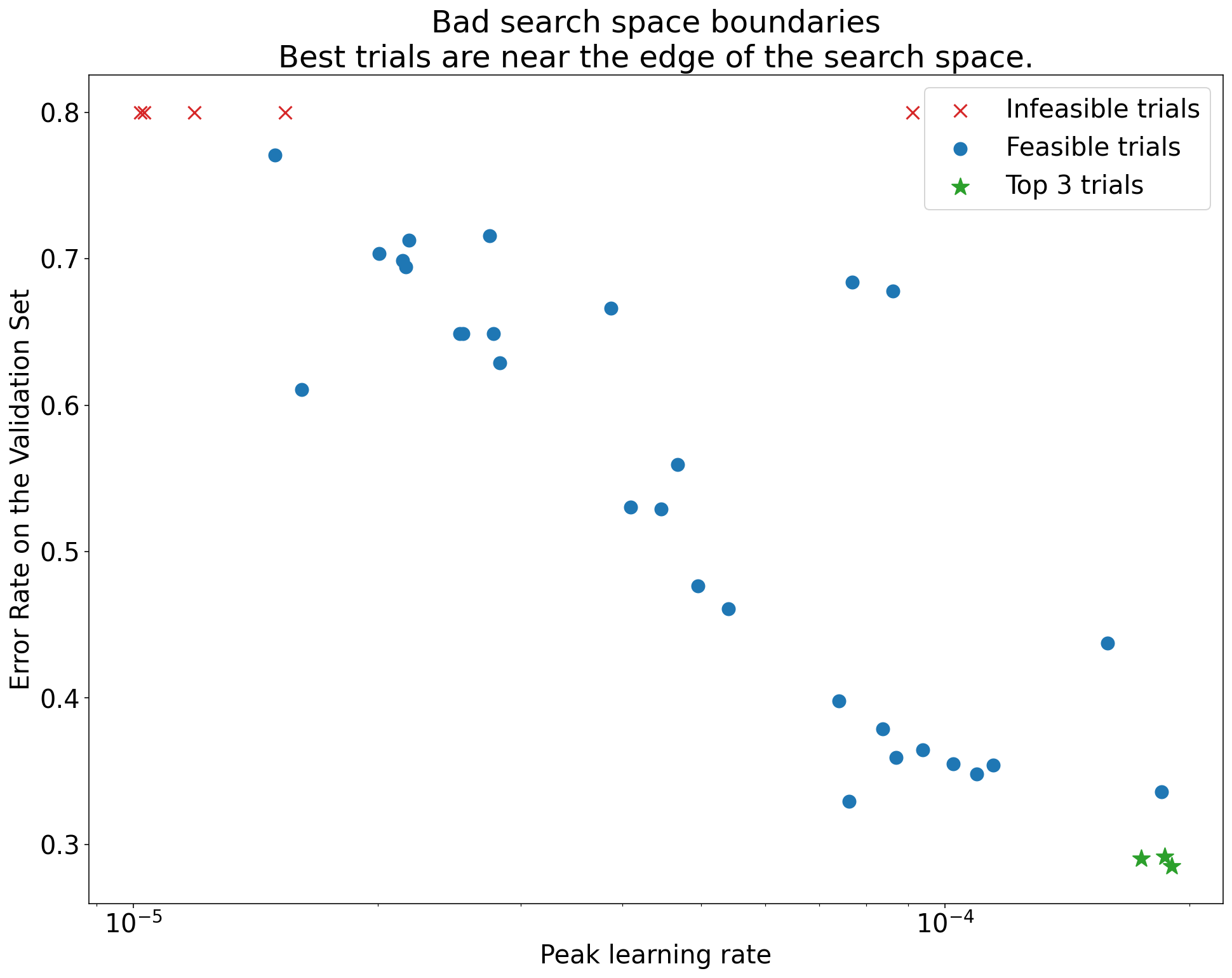
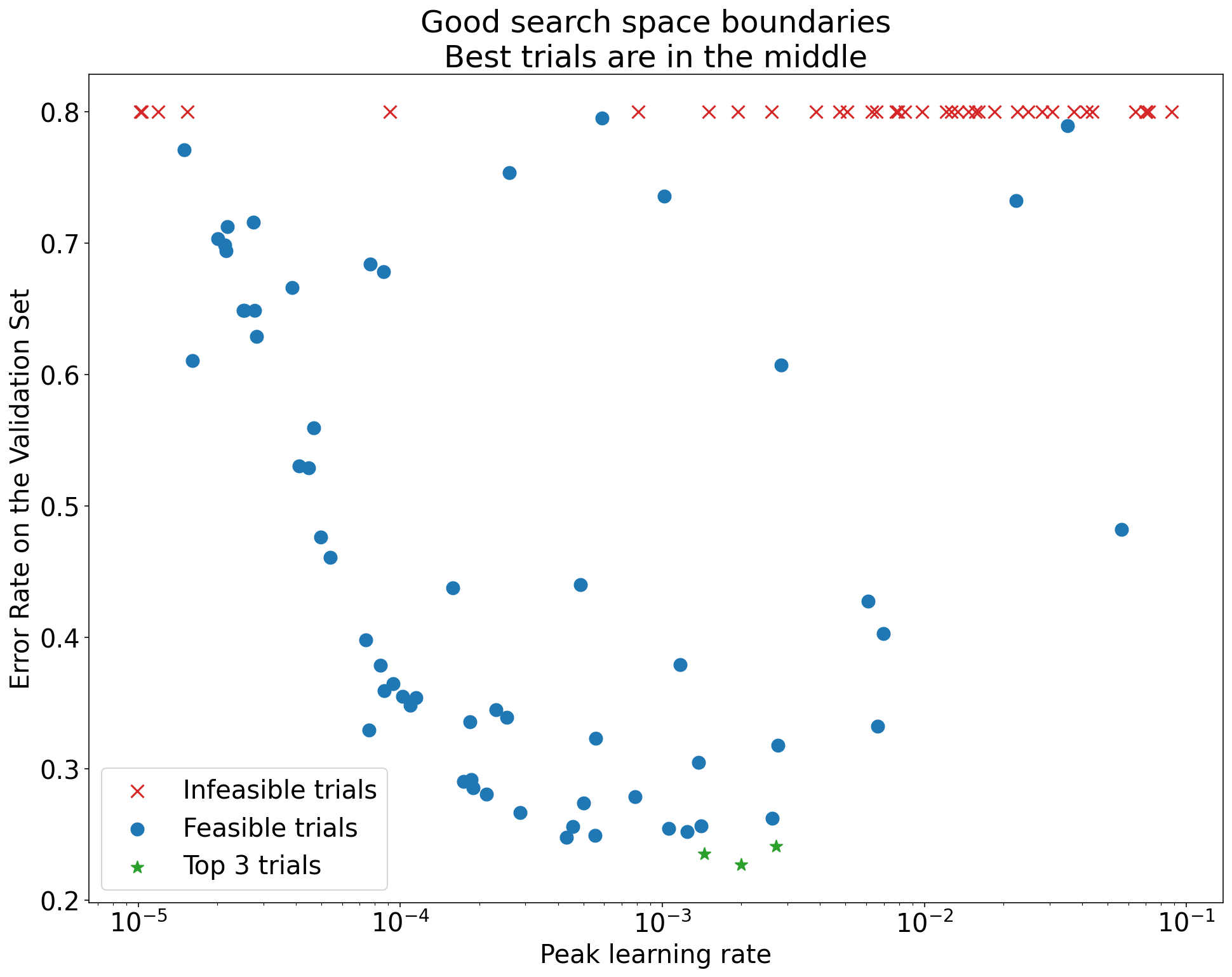
Figure 1: Examples of bad search space boundaries and acceptable search space boundaries.
The plots in Figure 1 show the error rate (lower is better) against the initial learning rate. If the best points cluster towards the edge of a search space (in some dimension), then you might need to expand the search space boundaries until the best observed point is no longer close to the boundary.
Often, a study includes "infeasible" trials that diverge or get very bad results (marked with red Xs in Figure 1). If all trials are infeasible for learning rates greater than some threshold value, and if the best performing trials have learning rates at the edge of that region, the model may suffer from stability issues preventing it from accessing higher learning rates.
Not sampling enough points in the search space
In general, it can be very difficult to know if the search space has been sampled densely enough. 🤖 Running more trials is better than running fewer trials, but more trials generates an obvious extra cost.
Since it is so hard to know when you have sampled enough, we recommend:
- Sampling what you can afford.
- Calibrating your intuitive confidence from repeatedly looking at various hyperparameter axis plots and trying to get a sense of how many points are in the "good" region of the search space.
Examine the training curves
Summary: Examining the loss curves is an easy way to identify common failure modes and can help you prioritize potential next actions.
In many cases, the primary objective of your experiments only requires considering the validation error of each trial. However, be careful when reducing each trial to a single number because that focus can hide important details about what's going on below the surface. For every study, we strongly recommend looking at the loss curves of at least the best few trials. Even if this is not necessary for addressing the primary experimental objective, examining the loss curves (including both training loss and validation loss) is a good way to identify common failure modes and can help you prioritize what actions to take next.
When examining the loss curves, focus on the following questions:
Are any of the trials exhibiting problematic overfitting? Problematic overfitting occurs when the validation error starts increasing during training. In experimental settings where you optimize away nuisance hyperparameters by selecting the "best" trial for each setting of the scientific hyperparameters, check for problematic overfitting in at least each of the best trials corresponding to the settings of the scientific hyperparameters that you're comparing. If any of the best trials exhibits problematic overfitting, do either or both of the following:
- Rerun the experiment with additional regularization techniques
- Retune the existing regularization parameters before comparing the values of the scientific hyperparameters. This may not apply if the scientific hyperparameters include regularization parameters, since then it wouldn't be surprising if low-strength settings of those regularization parameters resulted in problematic overfitting.
Reducing overfitting is often straightforward using common regularization techniques that add minimal code complexity or extra computation (for example, dropout regularization, label smoothing, weight decay). Therefore, it's usually trivial to add one or more of these to the next round of experiments. For example, if the scientific hyperparameter is "number of hidden layers" and the best trial that uses the largest number of hidden layers exhibits problematic overfitting, then we recommend retrying with additional regularization instead of immediately selecting the smaller number of hidden layers.
Even if none of the "best" trials exhibit problematic overfitting, there might still be a problem if it occurs in any of the trials. Selecting the best trial suppresses configurations exhibiting problematic overfitting and favors those that don't. In other words, selecting the best trial favors configurations with more regularization. However, anything that makes training worse can act as a regularizer, even if it wasn't intended that way. For example, choosing a smaller learning rate can regularize training by hobbling the optimization process, but we typically don't want to choose the learning rate this way. Note that the "best" trial for each setting of the scientific hyperparameters might be selected in such a way that favors "bad" values of some of the scientific or nuisance hyperparameters.
Is there high step-to-step variance in the training or validation error late in training? If so, this could interfere with both of the following:
- Your ability to compare different values of the scientific hyperparameters. That's because each trial randomly ends on a "lucky" or "unlucky" step.
- Your ability to reproduce the result of the best trial in production. That's because the production model might not end on the same "lucky" step as in the study.
The most likely causes of step-to-step variance are:
- Batch variance due to randomly sampling examples from the training set for each batch.
- Small validation sets
- Using a learning rate that's too high late in training.
Possible remedies include:
- Increasing the batch size.
- Obtaining more validation data.
- Using learning rate decay.
- Using Polyak averaging.
Are the trials still improving at the end of training? If so, you are in the "compute bound" regime and may benefit from increasing the number of training steps or changing the learning rate schedule.
Has performance on the training and validation sets saturated long before the final training step? If so, this indicates that you are in the "not compute-bound" regime and that you may be able to decrease the number of training steps.
Beyond this list, many additional behaviors can become evident from examining the loss curves. For example, training loss increasing during training usually indicates a bug in the training pipeline.
Detecting whether a change is useful with isolation plots
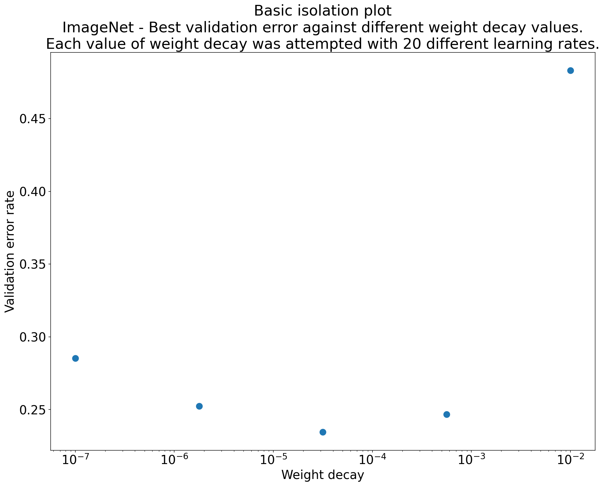
Figure 2: Isolation plot that investigates the best value of weight decay for ResNet-50 trained on ImageNet.
Often, the goal of a set of experiments is to compare different values of a scientific hyperparameter. For example, suppose you want to determine the value of weight decay that results in the best validation error. An isolation plot is a special case of the basic hyperparameter axis plot. Each point on an isolation plot corresponds to the performance of the best trial across some (or all) of the nuisance hyperparameters. In other words, plot the model performance after "optimizing away" the nuisance hyperparameters.
An isolation plot simplifies performing an apples-to-apples comparison between different values of the scientific hyperparameter. For example, the isolation plot in Figure 2 reveals the value of weight decay that produces the best validation performance for a particular configuration of ResNet-50 trained on ImageNet.
If the goal is to determine whether to include weight decay at all, then compare the best point from this plot against the baseline of no weight decay. For a fair comparison, the baseline should also have its learning rate equally well tuned.
When you have data generated by (quasi)random search and are considering a continuous hyperparameter for an isolation plot, you can approximate the isolation plot by bucketing the x-axis values of the basic hyperparameter axis plot and taking the best trial in each vertical slice defined by the buckets.
Automate generically useful plots
The more effort it is to generate plots, the less likely you are to look at them as much as you should. Therefore, we recommend setting up your infrastructure to automatically produce as many plots as possible. At a minimum, we recommend automatically generating basic hyperparameter axis plots for all hyperparameters that you vary in an experiment.
Additionally, we recommend automatically producing loss curves for all trials. Furthermore, we recommend making it as easy as possible to find the best few trials of each study and to examine their loss curves.
You can add many other useful potential plots and visualizations. To paraphrase Geoffrey Hinton:
Every time you plot something new, you learn something new.
Determine whether to adopt the candidate change
Summary: When deciding whether to make a change to our model or training procedure or adopt a new hyperparameter configuration, note the different sources of variation in your results.
When trying to improve a model, a particular candidate change might initially achieve a better validation error compared to an incumbent configuration. However, repeating the experiment might demonstrate no consistent advantage. Informally, the most important sources of inconsistent results can be grouped into the following broad categories:
- Training procedure variance, retrain variance, or trial variance: the variation between training runs that use the same hyperparameters but different random seeds. For example, different random initializations, training data shuffles, dropout masks, patterns of data augmentation operations, and orderings of parallel arithmetic operations are all potential sources of trial variance.
- Hyperparameter search variance, or study variance: the variation in results caused by our procedure to select the hyperparameters. For example, you might run the same experiment with a particular search space but with two different seeds for quasi-random search and end up selecting different hyperparameter values.
- Data collection and sampling variance: the variance from any sort of random split into training, validation, and test data or variance due to the training data generation process more generally.
True, you can compare validation error rates estimated on a finite validation set using fastidious statistical tests. However, often the trial variance alone can produce statistically significant differences between two different trained models that use the same hyperparameter settings.
We are most concerned about study variance when trying to make conclusions that go beyond the level of an individual point in hyperparameters space. The study variance depends on the number of trials and the search space. We have seen cases where the study variance is larger than the trial variance and cases where it is much smaller. Therefore, before adopting a candidate change, consider running the best trial N times to characterize the run-to-run trial variance. Usually, you can get away with only recharacterizing the trial variance after major changes to the pipeline, but you might need fresher estimates in some cases. In other applications, characterizing the trial variance is too costly to be worth it.
Although you only want to adopt changes (including new hyperparameter configurations) that produce real improvements, demanding complete certainty that a given change helps isn't the right answer either. Therefore, if a new hyperparameter point (or other change) gets a better result than the baseline (taking into account the retrain variance of both the new point and the baseline as best as you can), then you probably should adopt it as the new baseline for future comparisons. However, we recommend only adopting changes that produce improvements that outweigh any complexity they add.
After exploration concludes
Summary: Bayesian optimization tools are a compelling option once you're done searching for good search spaces and have decided what hyperparameters are worth tuning.
Eventually, your priorities will shift from learning more about the tuning problem to producing a single best configuration to launch or otherwise use. At that point, there should be a refined search space that comfortably contains the local region around the best observed trial and has been adequately sampled. Your exploration work should have revealed the most essential hyperparameters to tune and their sensible ranges that you can use to construct a search space for a final automated tuning study using as large a tuning budget as possible.
Since you no longer care about maximizing insight into the tuning problem, many of the advantages of quasi-random search no longer apply. Therefore, you should use Bayesian optimization tools to automatically find the best hyperparameter configuration. Open-Source Vizier implements a variety of sophisticated algorithms for tuning ML models, including Bayesian Optimization algorithms.
Suppose the search space contains a non-trivial volume of divergent points, meaning points that get NaN training loss or even training loss many standard deviations worse than the mean. In this case, we recommend using black-box optimization tools that properly handle trials that diverge. (See Bayesian Optimization with Unknown Constraints for an excellent way to deal with this issue.) Open-Source Vizier has supports for marking divergent points by marking trials as infeasible, although it may not use our preferred approach from Gelbart et al., depending on how it is configured.
After exploration concludes, consider checking the performance on the test set. In principle, you could even fold the validation set into the training set and retrain the best configuration found with Bayesian optimization. However, this is only appropriate if there won't be future launches with this specific workload (for example, a one-time Kaggle competition).