Page Summary
-
Optimization failures should be addressed before other debugging steps, as training instability can significantly impact model performance.
-
Training instabilities can be identified by observing loss curves at learning rates above the optimal rate and by monitoring the gradient norm.
-
Common solutions for training instability include learning rate warmup, gradient clipping, choosing a different optimizer, and ensuring best architectural practices.
-
Learning rate warmup involves gradually increasing the learning rate to a stable point, which can mitigate early training instability.
-
Gradient clipping limits the magnitude of gradients, preventing sudden spikes that can cause instability during training.
How can optimization failures be debugged and mitigated?
Summary: If the model is experiencing optimization difficulties, it's important to fix them before trying other things. Diagnosing and correcting training failures is an active area of research.
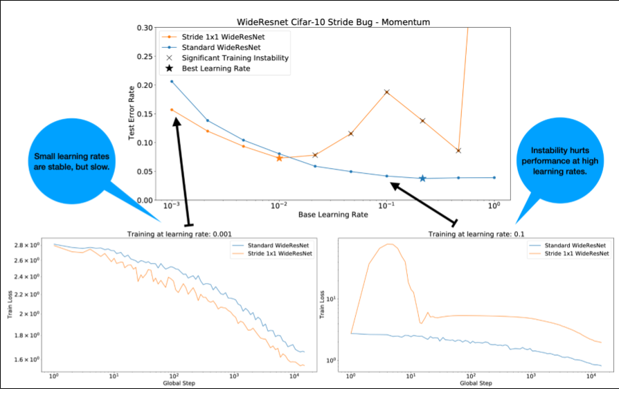
Notice the following about Figure 4:
- Changing the strides does not degrade performance at low learning rates.
- High learning rates no longer train well due to the instability.
- Applying 1000 steps of learning rate warmup resolves this particular instance of instability, allowing stable training at max learning rate of 0.1.
Identifying unstable workloads
Any workload becomes unstable if the learning rate is too large. Instability is only an issue when it forces you to use a learning rate that's too small. At least two types of training instability are worth distinguishing:
- Instability at initialization or early in training.
- Sudden instability in the middle of training.
You can take a systematic approach to identifying stability issues in your workload by doing the following:
- Do a learning rate sweep and find the best learning rate lr*.
- Plot training loss curves for learning rates just above lr*.
- If the learning rates > lr* show loss instability (loss goes up not down during periods of training), then fixing the instability typically improves training.
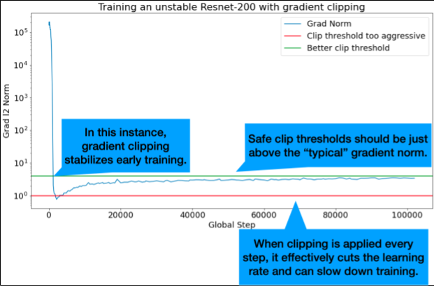
Log the L2 norm of the full loss gradient during training, since outlier values can cause spurious instability in the middle of training. This can inform how aggressively to clip gradients or weight updates.
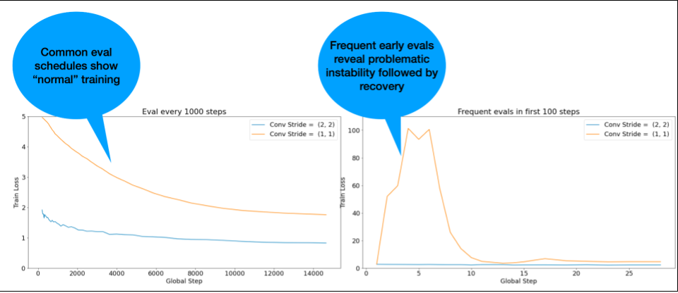
NOTE: Some models show very early instability followed by a recovery that results in slow but stable training. Common evaluation schedules can miss these issues by not evaluating frequently enough!
To check for this, you can train for an abbreviated run of just ~500 steps
using lr = 2 * current best, but evaluate every step.
Potential fixes for common instability patterns
Consider the following possible fixes for common instability patterns:
- Apply learning rate warmup. This is best for early training instability.
- Apply gradient clipping. This is good for both early and mid-training instability, and it may fix some bad initializations that warmup cannot.
- Try a new optimizer. Sometimes Adam can handle instabilities that Momentum can't. This is an active area of research.
- Ensure that you're using best practices and best initializations for your model architecture (examples to follow). Add residual connections and normalization if the model doesn't already contain them.
- Normalize as the last operation before the residual. For example:
x + Norm(f(x)). Note thatNorm(x + f(x))can cause issues. - Try initializing residual branches to 0. (See ReZero is All You Need: Fast Convergence at Large Depth.)
- Lower the learning rate. This is a last resort.
Learning rate warmup
When to apply learning rate warmup
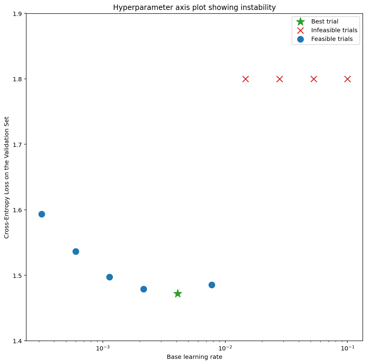
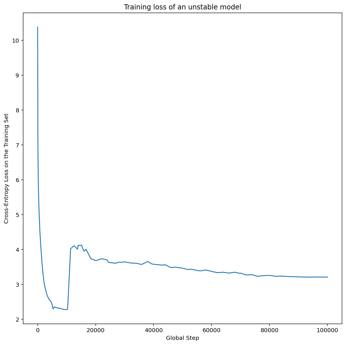
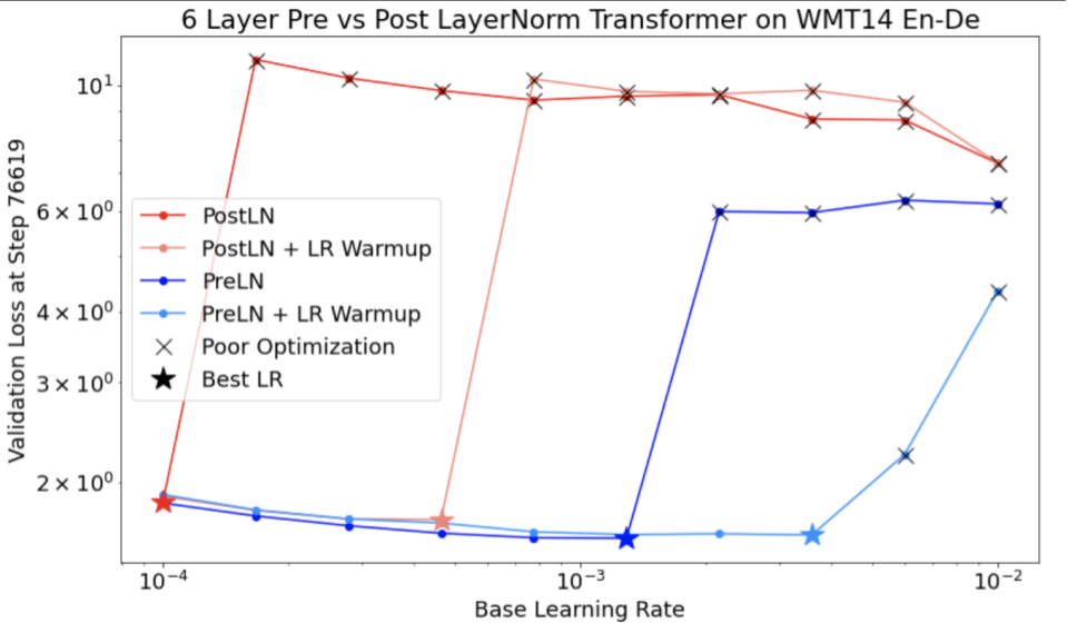
Figure 7a shows a hyperparameter axis plot that indicates a model experiencing optimization instabilities, because the best learning rate is right at the edge of instability.
Figure 7b shows how this can be double-checked by examining the training loss of a model trained with a learning rate either 5x or 10x larger than this peak. If that plot shows a sudden rise in the loss after a steady decline (e.g. at step ~10k in the figure above), then the model likely suffers from optimization instability.
How to apply learning rate warmup
Let unstable_base_learning_rate be the learning rate at which the model
becomes unstable, using the preceding procedure.
Warmup involves prepending a learning rate schedule that ramps up the
learning rate from 0 to some stable base_learning_rate that is at least
one order of magnitude larger than unstable_base_learning_rate.
The default would be to try a base_learning_rate that's 10x
unstable_base_learning_rate. Although note that it'd be possible to
run this entire procedure again for something like 100x
unstable_base_learning_rate. The specific schedule is:
- Ramp up from 0 to base_learning_rate over warmup_steps.
- Train at a constant rate for post_warmup_steps.
Your goal is to find the shortest number of warmup_steps that lets you
access peak learning rates that are much higher than
unstable_base_learning_rate.
So for each base_learning_rate, you need to tune warmup_steps and
post_warmup_steps. It's usually fine to set post_warmup_steps to be
2*warmup_steps.
Warmup can be tuned independently of an existing decay schedule. warmup_steps
should be swept at a few different orders of magnitude. For example, an
example study could try [10, 1000, 10,000, 100,000]. The largest feasible
point shouldn't be more than 10% of max_train_steps.
Once a warmup_steps that doesn't blow up training at base_learning_rate
has been established, it should be applied to the baseline model.
Essentially, prepend this schedule onto the existing schedule, and use
the optimal checkpoint selection discussed above to compare this experiment
to the baseline. For example, if we originally had 10,000 max_train_steps
and did warmup_steps for 1000 steps, the new training procedure should
run for 11,000 steps total.
If long warmup_steps are required for stable training (>5% of
max_train_steps), you might need to increase max_train_steps to account
for this.
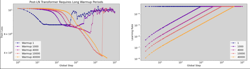
There isn't really a "typical" value across the full range of workloads. Some models only need 100 steps, while others (particularly transformers) may need 40k+.
Gradient clipping
Gradient clipping is most useful when large or outlier gradient issues occur. Gradient Clipping can fix either of the following problems:
- Early training instability (large gradient norm early)
- Mid-training instabilities (sudden gradient spikes mid training).
Sometimes longer warmup periods can correct instabilities that clipping does not; for details, see Learning rate warmup.
🤖 What about clipping during warmup?
The ideal clip thresholds are just above the "typical" gradient norm.
Here's an example of how gradient clipping could be done:
- If the norm of the gradient $\left | g \right |$ is greater than the gradient clipping threshold $\lambda$, then do ${g}'= \lambda \times \frac{g}{\left | g \right |}$ where ${g}'$ is the new gradient.
Log the unclipped gradient norm during training. By default, generate:
- A plot of gradient norm vs step
- A histogram of gradient norms aggregated over all steps
Choose a gradient clipping threshold based on the 90th percentile of gradient norms. The threshold is workload dependent, but 90% is a good starting point. If 90% doesn't work, you can tune this threshold.
🤖 What about some sort of adaptive strategy?
If you try gradient clipping and the instability issues remain, you can try it harder; that is, you can make the threshold smaller.
Extremely aggressive gradient clipping (that is, >50% of the updates getting clipped), is, in essence, a strange way of reducing the learning rate. If you find yourself using extremely aggressive clipping, you probably should just cut the learning rate instead.
Why do you call the learning rate and other optimization parameters hyperparameters? They are not parameters of any prior distribution.
The term "hyperparameter" has a precise meaning in Bayesian machine learning, so referring to learning rate and most of the other tunable deep learning parameters as "hyperparameters" is arguably an abuse of terminology. We would prefer to use the term "metaparameter" for learning rates, architectural parameters, and all the other tunable things deep learning. That's because metaparameter avoids the potential for confusion that comes from misusing the word "hyperparameter." This confusion is especially likely when discussing Bayesian optimization, where the probabilistic response surface models have their own true hyperparameters.
Unfortunately, although potentially confusing, the term "hyperparameter" has become extremely common in the deep learning community. Therefore, for this document, intended for a wide audience that includes many people who are unlikely to be aware of this technicality, we made the choice to contribute to one source of confusion in the field in hopes of avoiding another. That said, we might make a different choice when publishing a research paper, and we would encourage others to use "metaparameter" instead in most contexts.
Why shouldn't the batch size be tuned to directly improve validation set performance?
Changing the batch size without changing any other details of the training pipeline often affects the validation set performance. However, the difference in validation set performance between two batch sizes typically goes away if the training pipeline is optimized independently for each batch size.
The hyperparameters that interact most strongly with the batch size, and therefore are most important to tune separately for each batch size, are the optimizer hyperparameters (for example, learning rate, momentum) and the regularization hyperparameters. Smaller batch sizes introduce more noise into the training algorithm due to sample variance. This noise can have a regularizing effect. Thus, larger batch sizes can be more prone to overfitting and may require stronger regularization and/or additional regularization techniques. In addition, you might need to adjust the number of training steps when changing the batch size.
Once all these effects are taken into account, there is no convincing evidence that the batch size affects the maximum achievable validation performance. For details, see Shallue et al. 2018.
What are the update rules for all the popular optimization algorithms?
This section provides updates rules for several popular optimization algorithms.
Stochastic gradient descent (SGD)
\[\theta_{t+1} = \theta_{t} - \eta_t \nabla \mathcal{l}(\theta_t)\]
Where $\eta_t$ is the learning rate at step $t$.
Momentum
\[v_0 = 0\]
\[v_{t+1} = \gamma v_{t} + \nabla \mathcal{l}(\theta_t)\]
\[\theta_{t+1} = \theta_{t} - \eta_t v_{t+1}\]
Where $\eta_t$ is the learning rate at step $t$, and $\gamma$ is the momentum coefficient.
Nesterov
\[v_0 = 0\]
\[v_{t+1} = \gamma v_{t} + \nabla \mathcal{l}(\theta_t)\]
\[\theta_{t+1} = \theta_{t} - \eta_t ( \gamma v_{t+1} + \nabla \mathcal{l}(\theta_{t}) )\]
Where $\eta_t$ is the learning rate at step $t$, and $\gamma$ is the momentum coefficient.
RMSProp
\[v_0 = 1 \text{, } m_0 = 0\]
\[v_{t+1} = \rho v_{t} + (1 - \rho) \nabla \mathcal{l}(\theta_t)^2\]
\[m_{t+1} = \gamma m_{t} + \frac{\eta_t}{\sqrt{v_{t+1} + \epsilon}}\nabla \mathcal{l}(\theta_t)\]
\[\theta_{t+1} = \theta_{t} - m_{t+1}\]
ADAM
\[m_0 = 0 \text{, } v_0 = 0\]
\[m_{t+1} = \beta_1 m_{t} + (1 - \beta_1) \nabla \mathcal{l} (\theta_t)\]
\[v_{t+1} = \beta_2 v_{t} + (1 - \beta_2) \nabla \mathcal{l}(\theta_t)^2\]
\[b_{t+1} = \frac{\sqrt{1 - \beta_2^{t+1}}}{1 - \beta_1^{t+1}}\]
\[\theta_{t+1} = \theta_{t} - \alpha_t \frac{m_{t+1}}{\sqrt{v_{t+1}} + \epsilon} b_{t+1}\]
NADAM
\[m_0 = 0 \text{, } v_0 = 0\]
\[m_{t+1} = \beta_1 m_{t} + (1 - \beta_1) \nabla \mathcal{l} (\theta_t)\]
\[v_{t+1} = \beta_2 v_{t} + (1 - \beta_2) \nabla \mathcal{l} (\theta_t)^2\]
\[b_{t+1} = \frac{\sqrt{1 - \beta_2^{t+1}}}{1 - \beta_1^{t+1}}\]
\[\theta_{t+1} = \theta_{t} - \alpha_t \frac{\beta_1 m_{t+1} + (1 - \beta_1) \nabla \mathcal{l} (\theta_t)}{\sqrt{v_{t+1}} + \epsilon} b_{t+1}\]