此词汇表定义了人工智能术语。
A
消融
一种用于评估特征或组件重要性的技术,方法是将相应特征或组件暂时从模型中移除。然后,您可以在不使用该特征或组件的情况下重新训练模型,如果重新训练后的模型性能明显下降,则表明移除的特征或组件可能很重要。
例如,假设您使用 10 个特征训练了一个分类模型,并在测试集上实现了 88% 的精确率。如需检查第一个特征的重要性,您可以仅使用其他 9 个特征重新训练模型。如果重新训练后的模型性能明显下降(例如,精确率为 55%),则表明移除的特征可能很重要。反之,如果重新训练后的模型表现同样出色,则该特征可能并不那么重要。
消融还可以帮助确定以下各项的重要性:
- 较大的组件,例如大型机器学习系统的整个子系统
- 流程或技术,例如数据预处理步骤
在这两种情况下,您都会观察到在移除组件后,系统的性能会发生怎样的变化(或不发生变化)。
A/B 测试
一种比较两种(或更多种)技术(即 A 和 B)的统计方法。通常,A 是现有技术,而 B 是新技术。A/B 测试不仅可以确定哪种技术的效果更好,还可以确定这种差异是否具有统计显著性。
A/B 测试通常会比较两种技术在单个指标上的表现;例如,两种技术在模型准确率方面的比较结果如何?不过,A/B 测试也可以比较任意有限数量的指标。
加速器芯片
一类专门的硬件组件,旨在执行深度学习算法所需的主要计算。
与通用 CPU 相比,加速器芯片(简称加速器)可以显著提高训练和推理任务的速度和效率。它们非常适合训练神经网络和处理类似的计算密集型任务。
加速器芯片的示例包括:
- Google 的张量处理单元 (TPU),具有专用于深度学习的硬件。
- NVIDIA 的 GPU 虽然最初是为图形处理而设计的,但旨在实现并行处理,从而显著提高处理速度。
准确性
正确的分类预测数量除以预测总数。具体来说:
例如,如果某个模型做出了 40 次正确预测和 10 次错误预测,那么其准确率为:
二元分类为不同类别的正确预测和错误预测提供了具体名称。因此,二元分类的准确率公式如下:
其中:
如需了解详情,请参阅机器学习速成课程中的分类:准确率、召回率、精确率和相关指标。
act
智能体循环中的一个阶段,在此阶段中,智能体会执行在推理阶段选择的操作。例如,行动阶段可以发送 API 请求。
action
在强化学习中,智能体在环境的状态之间转换的机制。智能体使用政策选择操作。
行动空间
代理可用于执行任务的一组资源。操作空间可能包括智能体可以调用的工具和 API,以及智能体拥有的权限。 一般来说,动作空间应足够大,以便智能体执行任务。如果动作空间过小,智能体可能没有足够的资源来执行任务。如果动作空间过大,智能体往往更容易出错。
激活函数
一种函数,可使神经网络能够学习特征与标签之间的非线性(复杂)关系。
常用的激活函数包括:
激活函数的图从不是单条直线。 例如,ReLU 激活函数的图由两条直线组成:

Sigmoid 激活函数的图如下所示:

点击相应图标即可查看示例。
在神经网络中,激活函数会处理神经元的所有输入的加权和。为了计算加权和,神经元会将相关值和权重的乘积相加。例如,假设某个神经元的相关输入包含以下内容:
| 输入值 | 输入权重 |
| 2 | -1.3 |
| -1 | 0.6 |
| 3 | 0.4 |
weighted sum = (2)(-1.3) + (-1)(0.6) + (3)(0.4) = -2.0

如需了解详情,请参阅机器学习速成课程中的神经网络:激活函数。
主动学习
一种训练方法,采用这种方法时,算法会选择从中学习规律的部分数据。当有标签样本稀缺或获取成本高昂时,主动学习尤其有用。主动学习算法会选择性地寻找学习所需的特定范围的样本,而不是盲目地寻找各种各样的有标签样本。
AdaGrad
一种先进的梯度下降法,用于重新调整每个形参的梯度,以便有效地为每个形参指定独立的学习速率。如需查看完整说明,请参阅用于在线学习和随机优化的自适应次梯度方法。
改编
与调优或微调的含义相同。
代理
能够对用户输入进行推理,以便代表用户规划和执行操作的软件。
在强化学习中,智能体是使用政策来最大限度提高从环境的状态转换中获得的预期回报的实体。
代理型
agent 的形容词形式。Agentic 是指智能体所具备的特质(例如自主性)。
智能体循环
智能体反复执行的循环,直到满足终止条件。该周期通常包括以下四个阶段:
智能体工作流
一种动态流程,其中智能体自主规划和执行行动以实现目标。该过程可能涉及推理、调用外部工具和自行纠正方案。
智能体编排
跨多个子代理或 LLM 调用的任务的集中管理和路由。智能体编排功能可将复杂任务分解为更小的子任务,并将其分配给最能胜任的子智能体。
凝聚式层次聚类
请参阅层次聚类。
AI 生成的垃圾
生成式 AI 系统生成的输出,侧重于数量而非质量。例如,包含 AI 生成的垃圾的网页充斥着低成本制作的 AI 生成的低质量内容。
异常值检测
识别离群点的过程。例如,如果某个特征的平均值为 100,标准差为 10,那么异常检测功能应将 200 的值标记为可疑。
AR
增强现实的缩写。
PR 曲线下的面积
ROC 曲线下面积
请参阅 AUC(ROC 曲线下面积)。
人工通用智能
一种非人类机制,可展现广泛的问题解决能力、创造力和适应性。例如,展示通用人工智能的程序可以翻译文本、创作交响乐,并在尚未发明的游戏中表现出色。
人工智能
能够解决复杂任务的非人类程序或模型。 例如,翻译文本的程序或模型,以及根据放射影像识别疾病的程序或模型都展现出了人工智能。
从形式上讲,机器学习是人工智能的一个子领域。不过,近年来,一些组织开始交替使用人工智能和机器学习这两个术语。
Attention
一种用于神经网络的机制,用于指示特定字词或字词部分的重要性。注意力机制可压缩模型预测下一个 token/字词所需的信息量。典型的注意力机制可能包含一组输入的加权和,其中每个输入的权重由神经网络的另一部分计算得出。
另请参阅 自注意力机制和多头自注意力机制,它们是 Transformer 的构建块。
如需详细了解自注意力机制,请参阅机器学习速成课程中的 LLM:什么是大语言模型?。
属性
与特征的含义相同。
在机器学习公平性方面,属性通常是指与个人相关的特征。
属性抽样
一种用于训练决策森林的策略,其中每个决策树在学习条件时仅考虑随机选择的可能特征子集。一般来说,每个节点都会对不同的特征子集进行抽样。相比之下,在训练不进行属性抽样的决策树时,系统会考虑每个节点的所有可能特征。
AUC(ROC 曲线下面积)
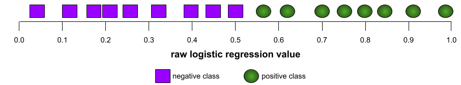
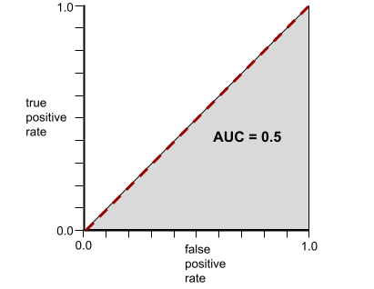
一个介于 0.0 和 1.0 之间的数字,表示二元分类模型区分正类别和负类别的能力。 AUC 越接近 1.0,模型区分不同类别的能力就越好。
例如,下图展示了一个完美区分正类别(绿色椭圆)和负类别(紫色矩形)的分类模型。这个不切实际的完美模型的 AUC 为 1.0:
相反,下图显示了生成随机结果的分类模型的结果。此模型的 AUC 为 0.5:
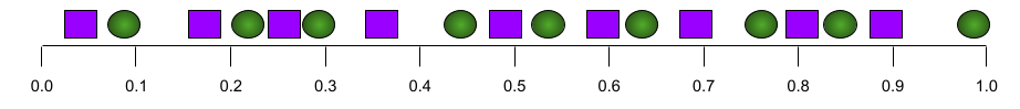
是的,上述模型的 AUC 为 0.5,而不是 0.0。
大多数模型都介于这两个极端之间。例如,以下模型在一定程度上区分了正例和负例,因此其 AUC 介于 0.5 和 1.0 之间:
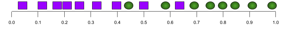
AUC 会忽略您为分类阈值设置的任何值。相反,AUC 会考虑所有可能的分类阈值。
点击该图标可了解 AUC 与 ROC 曲线之间的关系。
AUC 表示 ROC 曲线下的面积。例如,可完美区分正例和负例的模型的 ROC 曲线如下所示:
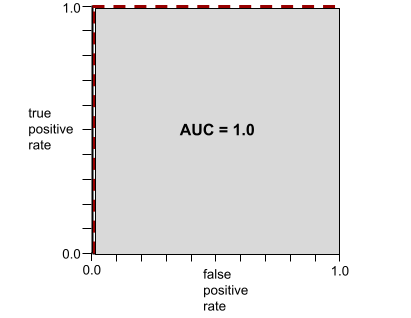
AUC 是上图中的灰色区域的面积。 在这种特殊情况下,面积就是灰色区域的长度 (1.0) 乘以灰色区域的宽度 (1.0)。因此,1.0 与 1.0 的乘积得到的曲线下面积正好是 1.0,这是最高的曲线下面积得分。
相反,完全无法区分类别的分类模型的 ROC 曲线如下所示。此灰色区域的面积为 0.5。
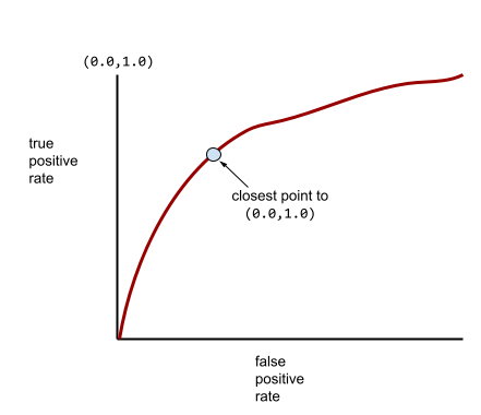
更典型的 ROC 曲线大致如下所示:
手动计算此曲线下的面积非常费力,因此通常由程序计算大多数 AUC 值。
如需了解详情,请参阅机器学习速成课程中的分类:ROC 和 AUC。
增强现实
一种将计算机生成的图像叠加到用户看到的真实世界上的技术,从而提供合成视图。
自动编码器
一种可学习从输入中提取最重要信息的系统。自动编码器是编码器和解码器的组合。自动编码器依赖于以下两步流程:
- 编码器将输入映射到(通常)有损的低维(中间)格式。
- 解码器通过将低维格式映射到原始高维输入格式来构建原始输入的有损版本。
通过让解码器尝试尽可能准确地从编码器的中间格式重建原始输入,对自动编码器进行端到端训练。由于中间格式比原始格式小(维度更低),因此自动编码器必须学习输入中哪些信息是必不可少的,并且输出不会与输入完全相同。
例如:
- 如果输入数据是图形,则非精确复制的图形与原始图形类似,但会进行一些修改。可能非精确副本会去除原始图形中的噪声或填充一些缺失的像素。
- 如果输入数据是文本,自动编码器会生成模仿(但不等同于)原始文本的新文本。
另请参阅变分自编码器。
自动评估
使用软件来判断模型输出的质量。
如果模型输出相对简单,脚本或程序可以将模型输出与标准回答进行比较。这种类型的自动评估有时称为程序化评估。ROUGE 或 BLEU 等指标通常有助于进行程序化评估。
如果模型输出复杂或没有唯一正确的答案,则有时会由一个名为自动评分器的单独机器学习程序执行自动评估。
与人工评估相对。
自动化偏差
是指针对自动化决策系统所给出的建议的偏差,在此偏差范围内,即使系统出现错误,决策者也会优先考虑自动化决策系统给出的建议,而不是非自动化系统给出的建议。
如需了解详情,请参阅机器学习速成课程中的公平性:偏差类型。
AutoML
用于构建机器学习 模型的任何自动化流程。AutoML 可以自动执行以下任务:
AutoML 对数据科学家很有用,因为它可以节省他们开发机器学习流水线的时间和精力,并提高预测准确率。对于非专业人士,它也很有用,因为它可以让他们更轻松地完成复杂的机器学习任务。
如需了解详情,请参阅机器学习速成课程中的自动化机器学习 (AutoML)。
自主智能体
一种通过规划、行动和适应来达成复杂目标的智能体,无需持续的人工干预。
自动评估器评估
一种用于评判生成式 AI 模型输出质量的混合机制,它将人工评估与自动评估相结合。自动评估器是一种基于人工评估生成的数据训练的机器学习模型。理想情况下,自动评估器会学习模仿人类评估者。虽然有预建的自动评分器,但最好是专门针对您要评估的任务进行微调的自动评分器。
自回归模型
一种模型,可根据其自身的先前预测推断预测结果。例如,自回归语言模型会根据之前预测的 token 来预测下一个 token。所有基于 Transformer 的大语言模型都是自回归模型。
相比之下,基于 GAN 的图像模型通常不是自回归的,因为它们通过一次前向传递生成图片,而不是以迭代方式分步生成图像。不过,某些图片生成模型是自回归模型,因为它们会分步生成图片。
辅助损失
一种与神经网络 模型的主要损失函数结合使用的损失函数,有助于在权重随机初始化的早期迭代期间加速训练。
辅助损失函数会将有效梯度推送到更早的层。这有助于通过解决梯度消失问题,在训练期间实现收敛。
前 k 名的平均精确率
一种用于总结模型在生成排名结果(例如图书推荐的编号列表)的单个提示上的表现的指标。k 处的平均精确率是指每个相关结果的k 处精确率值的平均值。 因此,前 k 个结果的平均精确率的公式为:
\[{\text{average precision at k}} = \frac{1}{n} \sum_{i=1}^n {\text{precision at k for each relevant item} } \]
其中:
- \(n\) 是列表中的相关商品数量。
与 k 处的召回率相对。
轴对齐条件
在决策树中,仅涉及单个特征的条件。例如,如果 area 是一个特征,则以下是轴对齐条件:
area > 200
与斜条件相对。
B
反向传播
训练神经网络需要多次迭代以下双向传递周期:
- 在前向传递期间,系统会处理一个包含 个示例的批次,以生成预测结果。系统会将每个预测值与每个标签值进行比较。预测值与标签值之间的差值就是相应示例的损失。系统会汇总所有示例的损失,以计算当前批次的总损失。
- 在反向传递(反向传播)期间,系统会通过调整所有隐藏层中所有神经元的权重来减少损失。
神经网络通常包含多个隐藏层中的许多神经元。每个神经元以不同的方式影响总体损失。 反向传播算法会确定是增加还是减少应用于特定神经元的权重。
学习速率是一种乘数,用于控制每次向后传递时每个权重增加或减少的程度。与较小的学习速率相比,较大的学习速率会更大幅度地增加或减少每个权重。
从微积分的角度来看,反向传播实现了微积分中的链式法则。也就是说,反向传播会计算误差相对于每个参数的偏导数。
多年前,机器学习从业者必须编写代码才能实现反向传播。Keras 等现代机器学习 API 现在会为您实现反向传播。好,
如需了解详情,请参阅机器学习速成课程中的神经网络。
装袋
一种用于训练集成的方法,其中每个组成模型都基于有放回抽样的随机训练示例子集进行训练。例如,随机森林是使用 Bagging 训练的决策树的集合。
术语“bagging”是“bootstrap aggregating”(自助抽样集成)的简称。
如需了解详情,请参阅“决策森林”课程中的随机森林。
词袋
词组或段落中的字词的表示法,不考虑字词顺序。例如,以下三个词组的词袋完全一样:
- the dog jumps
- jumps the dog
- dog jumps the
每个字词都映射到稀疏向量中的一个索引,其中词汇表中的每个字词都在该向量中有一个索引。例如,词组“the dog jumps”会映射到一个特征向量,该特征向量在字词“the”“dog”和“jumps”对应的三个索引处包含非零值。非零值可以是以下任一值:
- 1,表示某个字词存在。
- 某个字词出现在词袋中的次数。例如,如果词组为“the maroon dog is a dog with maroon fur”,那么“maroon”和“dog”都会表示为 2,其他字词则表示为 1。
- 其他一些值,例如,某个字词出现在词袋中的次数的对数。
baseline
一种用作参考点的模型,用于比较另一模型(通常是更复杂的模型)的效果。例如,逻辑回归模型可以作为深度模型的良好基准。
对于特定问题,基准有助于模型开发者量化新模型必须达到的最低预期性能,以便新模型发挥作用。
基础模型
一种预训练模型,可作为微调的起点,以解决特定任务或应用问题。
批处理
一次训练迭代中使用的示例集。批次大小决定了一个批次中的样本数量。
如需了解批次与周期之间的关系,请参阅周期。
如需了解详情,请参阅机器学习速成课程中的线性回归:超参数。
批量推理
对分为较小子集(“批次”)的多个无标签示例进行推理预测的过程。
批量推理可以利用加速器芯片的并行化功能。也就是说,多个加速器可以同时对不同批次未标记的示例进行推理预测,从而大幅提高每秒的推理次数。
如需了解详情,请参阅机器学习速成课程中的生产环境中的机器学习系统:静态推理与动态推理。
批次归一化
对隐藏层中激活函数的输入或输出进行归一化。批次归一化具有下列优势:
批次大小
一个批次中的样本数量。 例如,如果批次大小为 100,则模型在每次迭代中处理 100 个样本。
以下是常用的批次大小策略:
- 随机梯度下降法 (SGD),其中批次大小为 1。
- 完整批次,其中批次大小为整个训练集中的样本数量。例如,如果训练集包含 100 万个样本,则批次大小为 100 万个样本。完整批次通常是一种低效的策略。
- 小批次,其中批次大小通常介于 10 到 1000 之间。小批次通常是最有效的策略。
请参阅以下内容了解详细信息:
- 生产环境机器学习系统:静态推理与动态推理(机器学习速成课程)。
- 《深度学习调优指南》。
贝叶斯神经网络
一种概率神经网络,用于解释权重和输出的不确定性。标准神经网络回归模型通常会预测标量值;例如,某个标准模型预测房价为 853,000。相比之下,贝叶斯神经网络会预测值的分布情况;例如,某个贝叶斯模型预测房价为 853000,其中标准偏差为 67200。
贝叶斯神经网络根据 贝叶斯定理计算权重和预测的不确定性。如果需要量化不确定性,例如,在与医药相关的模型中,则贝叶斯神经网络非常有用。贝叶斯神经网络还有助于防止过拟合。
贝叶斯优化
一种概率回归模型技术,通过使用贝叶斯学习技术量化不确定性,优化计算成本高昂的目标函数,而不是直接优化目标函数。由于贝叶斯优化本身非常耗费资源,因此通常用于优化参数数量较少的评估成本较高的任务,例如选择超参数。
贝尔曼方程
在强化学习中,最优 Q 函数满足以下等式:
\[Q(s, a) = r(s, a) + \gamma \mathbb{E}_{s'|s,a} \max_{a'} Q(s', a')\]
强化学习算法应用此恒等式,使用以下更新规则创建 Q-learning:
\[Q(s,a) \gets Q(s,a) + \alpha \left[r(s,a) + \gamma \displaystyle\max_{\substack{a_1}} Q(s',a') - Q(s,a) \right] \]
除了强化学习之外,贝尔曼方程还可应用于动态规划。请参阅 维基百科中有关贝尔曼方程的条目。
BERT(基于 Transformer 的双向编码器表示法)
一种用于文本表示的模型架构。经过训练的 BERT 模型可以作为大型模型的一部分,用于文本分类或其他机器学习任务。
BERT 具有以下特征:
- 使用 Transformer 架构,因此依赖于自注意力。
- 使用 Transformer 的编码器部分。编码器的任务是生成良好的文本表示法,而不是执行分类等特定任务。
- 是否为双向。
- 使用遮盖进行无监督训练。
BERT 的变体包括:
如需简要了解 BERT,请参阅开源 BERT:最先进的自然语言处理预训练。
偏差(道德/公平性)
1. 对某些事物、人或群体有刻板印象、偏见或偏袒。这些偏差会影响数据的收集和解读、系统设计以及用户与系统的互动方式。此类偏差的形式包括:
2. 采样或报告过程中引入的系统性误差。 此类偏差的形式包括:
如需了解详情,请参阅机器学习速成课程中的公平性:偏差类型。
偏差(数学概念)或偏差项
距离原点的截距或偏移。偏差是机器学习模型中的一个形参,可用以下任一符号表示:
- b
- w0
例如,在下面的公式中,偏差为 b:
在简单的二维线性模型中,偏差只是指“y 轴截距”。 例如,下图中的直线的偏差为 2。
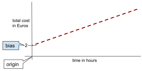
之所以存在偏差,是因为并非所有模型都从原点 (0,0) 开始。例如,假设某游乐园的门票为 2 欧元,客户每停留 1 小时需额外支付 0.5 欧元。因此,映射总费用的模型具有 2 的偏差,因为最低费用为 2 欧元。
如需了解详情,请参阅机器学习速成课程中的线性回归。
双向
一种用于描述评估目标文本部分之前和之后文本的系统的术语。相比之下,单向系统仅评估目标文本部分之前的文本。
例如,假设有一个遮盖式语言模型,它必须确定以下问题中带下划线的字词的概率:
你有什么_____?
单向语言模型必须仅根据“What”“is”和“the”这几个字词提供的上下文来确定概率。相比之下,双向语言模型还可以从“with”和“you”中获取上下文,这可能有助于模型生成更好的预测结果。
双向语言模型
一种语言模型,用于根据前文和后文确定给定 token 出现在文本摘录中给定位置的概率。
二元语法
一种 N 元语法,其中 N=2。
二元分类
一种分类任务,用于预测两个互斥的类别之一:
例如,以下两个机器学习模型都执行二元分类:
- 一种用于确定电子邮件是垃圾邮件(正类别)还是非垃圾邮件(负类别)的模型。
- 一种评估医疗症状以确定某人是否患有特定疾病(正类别)或未患有该疾病(负类别)的模型。
与多类别分类相对。
如需了解详情,请参阅机器学习速成课程中的分类。
二元条件
在决策树中,条件只有两种可能的结果,通常是是或否。例如,以下是一个二元条件:
temperature >= 100
与非二元条件相对。
如需了解详情,请参阅决策森林课程中的条件类型。
分箱
与分桶的含义相同。
黑盒模型
一种模型,其“推理”过程难以理解或无法理解。也就是说,虽然人类可以看到提示如何影响回答,但人类无法准确确定黑盒模型如何确定回答。换句话说,黑盒模型缺乏可解释性。
BLEU(双语替换评测)
一种介于 0.0 和 1.0 之间的指标,用于评估机器翻译的质量,例如从西班牙语到日语的翻译。
为了计算得分,BLEU 通常会将机器学习模型的翻译(生成的文本)与人类专家的翻译(参考文本)进行比较。生成文本和参考文本中 N 元语法的匹配程度决定了 BLEU 得分。
有关此指标的原始论文是《BLEU:一种用于自动评估机器翻译的方法》。
另请参阅 BLEURT。
BLEURT(基于 Transformer 的双语替换评测)
一种用于评估从一种语言到另一种语言(尤其是英语)的机器翻译的指标。
对于英语与另一种语言之间的翻译,BLEURT 与人工评分的契合度比 BLEU 更高。与 BLEU 不同,BLEURT 侧重于语义(含义)相似性,并且可以适应释义。
BLEURT 依赖于一个预训练的大语言模型(确切来说是 BERT),然后使用人工翻译人员提供的文本对该模型进行微调。
有关此指标的原始论文是 BLEURT: Learning Robust Metrics for Text Generation。
布尔值问题 (BoolQ)
一个用于评估 LLM 在回答是/否问题方面的熟练程度的数据集。 数据集中的每个挑战都包含三个组成部分:
- 查询
- 暗示查询答案的段落。
- 正确答案,即是或否。
例如:
- 问题:密歇根州有核电站吗?
- 段落:...three nuclear power plants supply Michigan with about 30% of its electricity.
- 正确答案:是
研究人员从匿名化的汇总 Google 搜索查询中收集问题,然后使用维基百科页面来确定信息。
如需了解详情,请参阅 BoolQ:探索自然是/否问题的惊人难度。
BoolQ 是 SuperGLUE 集成模型的一个组成部分。
BoolQ
布尔值问题的缩写。
增强学习
一种机器学习技术,以迭代方式将一组简单但不太准确的分类模型(也称为“弱分类器”)合成一个准确率高的分类模型(即“强分类器”),具体方法是对模型目前错误分类的样本进行权重上调。
如需了解详情,请参阅决策森林课程中的什么是梯度提升决策树?。
边界框
图片中感兴趣区域(例如下图中的狗)周围矩形的 (x, y) 坐标。

广播
将矩阵数学运算中某个运算数的形状扩展为与该运算兼容的维度。例如,线性代数要求矩阵加法运算中的两个运算数必须具有相同的维度。因此,您无法将形状为 (m, n) 的矩阵与长度为 n 的向量相加。为了使该运算有效,广播会在每列下复制相同的值,将长度为 n 的向量扩展成形状为 (m, n) 的矩阵。
如需了解详情,请参阅 NumPy 中的广播这篇文章的说明。
分桶
将单个特征转换为多个二元特征(称为桶或箱),通常根据值区间进行转换。截断特征通常是连续特征。
例如,您可以将温度范围划分为离散的区间,而不是将温度表示为单个连续的浮点特征,例如:
- ≤ 10 摄氏度为“寒冷”区间。
- 11-24 摄氏度为“温带”区间。
- >= 25 摄氏度为“温暖”区间。
模型将以相同方式处理同一分桶中的每个值。例如,值 13 和 22 都位于温和型分桶中,因此模型会以相同的方式处理这两个值。
如需了解详情,请参阅机器学习速成课程中的数值数据:分箱。
C
校准层
一种预测后调整,通常是为了降低预测偏差的影响。调整后的预测和概率应与观察到的标签集的分布一致。
候选集生成
推荐系统选择的初始推荐集。例如,假设某家书店有 10 万本书。在候选集生成阶段,推荐系统会针对特定用户生成一个小得多的合适书籍列表,比如 500 本。但即使向用户推荐 500 本也太多了。推荐系统的后续阶段(例如评分和重排序)会进一步将这 500 本书列表缩小为一个小得多且更实用的推荐集。
如需了解详情,请参阅推荐系统课程中的候选集生成概览。
候选采样
一种训练时进行的优化,会使用某种函数(例如 softmax)针对所有正类别标签计算概率,但仅随机抽取一部分负类别标签样本并计算概率。例如,给定一个标签为beagle和dog的实例,候选采样将针对以下类别计算预测概率和相应的损失项:
- beagle
- dog
- 其余负类别的随机子集(例如,猫、棒棒糖、栅栏)。
这种方法的理念是,只要正类别始终得到适当的正增强,负类别就可以从不太频繁的负增强中学习,这确实符合实际观察情况。
与计算所有负类别的预测结果的训练算法相比,候选采样在计算方面更高效,尤其是在负类别的数量非常庞大时。
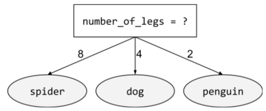
分类数据
特征,拥有一组特定的可能值。例如,假设有一个名为 traffic-light-state 的分类特征,该特征只能具有以下三个可能值之一:
redyellowgreen
通过将 traffic-light-state 表示为分类特征,模型可以了解 red、green 和 yellow 对驾驶员行为的不同影响。
分类特征有时称为离散特征。
与数值数据相对。
如需了解详情,请参阅机器学习速成课程中的处理分类数据。
因果语言模型
与单向语言模型的含义相同。
如需对比语言建模中的不同方向性方法,请参阅双向语言模型。
CB
CommitmentBank 的缩写。
形心
由 k-means 或 k-median 算法确定的聚类中心。例如,如果 k 为 3,则 k-means 或 k-median 算法会找出 3 个形心。
如需了解详情,请参阅聚类课程中的聚类算法。
形心聚类
一类聚类算法,用于将数据整理到非分层聚类中。k-means 是使用最广泛的形心聚类算法。
与层次聚类算法相对。
如需了解详情,请参阅聚类课程中的聚类算法。
思维链提示
一种提示工程技术,可鼓励大语言模型 (LLM) 逐步说明其推理过程。例如,请考虑以下提示,并特别注意第二句话:
如果一辆汽车从 0 加速到 60 英里/小时需要 7 秒,那么驾驶员会感受到多少 g 的重力?在回答中,显示所有相关计算。
LLM 的回答可能会:
- 显示一系列物理公式,并在适当的位置代入值 0、60 和 7。
- 说明系统为何选择这些公式,以及各种变量的含义。
思维链提示会强制 LLM 执行所有计算,这可能会得出更正确的答案。此外,通过思维链提示,用户可以检查 LLM 的步骤,以确定回答是否合理。
字符 N 元语法 F 得分 (ChrF)
用于评估机器翻译模型的指标。 字符 N 元语法 F 分数用于确定参考文本中 N 元语法与机器学习模型生成的文本中 N 元语法的重叠程度。
字符 N 元语法 F 分数与 ROUGE 和 BLEU 系列中的指标类似,但有以下区别:
- 字符 N 元语法 F 分数基于字符 N 元语法。
- ROUGE 和 BLEU 基于字词 N 元语法或令牌进行操作。
聊天
与机器学习系统(通常是大语言模型)进行来回对话的内容。 聊天中的上一次互动(您输入的内容以及大语言模型的回答)会成为聊天后续部分的上下文。
聊天机器人是大语言模型的一种应用。
检查点
用于捕获模型参数在训练期间或训练完成后的状态的数据。例如,在训练期间,您可以执行以下操作:
- 停止训练,可能是出于有意,也可能是由于某些错误。
- 捕获检查点。
- 稍后,重新加载检查点,可能是在不同的硬件上。
- 重新开始训练。
选择合理的替代方案 (COPA)
一个用于评估 LLM 在识别前提的两个备选答案中哪个更优方面的能力的数据集。数据集中的每个挑战都包含三个组成部分:
- 前提,通常是陈述后跟问题
- 前提中提出的问题的两种可能答案,其中一种正确,另一种不正确
- 正确答案
例如:
- 前提:该男子弄断了脚趾。导致这种情况的原因是什么?
- 可能的回答:
- 他的袜子破了个洞。
- 他把锤子掉在了脚上。
- 正确答案:2
COPA 是 SuperGLUE 集成模型的一个组成部分。
引用精确度
一种可回答以下问题的指标:
在 LLM 的回答中,有多少百分比的引用实际上是正确且具有支持性的?
也就是说,有多少百分比的引用包含验证 LLM 回答中所述声明所需的准确事实或相关信息。
例如,如果 LLM 回答引用了 10 份文档,但其中只有 7 份引用正确且具有支持性,那么引用精确率将为 0.7。
引用召回率
一种可回答以下问题的指标:
LLM 在撰写回答时使用的源文档中有多少百分比实际上在回答中被引用?
例如,如果 LLM 依赖 20 份文档来撰写回答,但回答仅引用了其中 11 份文档,那么引用召回率为 0.55。
类别
标签可以所属的类别。 例如:
分类模型可预测类别。 相比之下,回归模型预测的是数字,而不是类别。
如需了解详情,请参阅机器学习速成课程中的分类。
类别平衡的数据集
一个包含 分类 标签的数据集,其中每个类别的实例数量大致相等。例如,假设有一个植物学数据集,其二元标签可以是本地植物或非本地植物:
- 如果某个数据集包含 515 种本地植物和 485 种非本地植物,则该数据集属于类别平衡的数据集。
- 包含 875 种本地植物和 125 种非本地植物的数据集属于类别不平衡的数据集。
在类平衡数据集和类不平衡数据集之间没有明确的界限。只有当在高度类别不平衡的数据集上训练的模型无法收敛时,这种区别才变得重要。如需了解详情,请参阅机器学习速成课程中的数据集:不平衡的数据集。
分类模型
- 一个模型,用于预测输入句子的语言(法语?西班牙语? 意大利语?)。
- 一个模型,用于预测树种(枫树?橡树?猴面包树?)。
- 用于预测特定病症是阳性类别还是负类别的模型。
相比之下,回归模型预测的是数字,而不是类别。
以下是两种常见的分类模型:
分类阈值
在二元分类中,一个介于 0 到 1 之间的数字,用于将逻辑回归模型的原始输出转换为对正类别或负类别的预测。 请注意,分类阈值是人为选择的值,而不是通过模型训练选择的值。
逻辑回归模型会输出一个介于 0 到 1 之间的原始值。然后,执行以下操作:
- 如果此原始值大于分类阈值,则预测为正类别。
- 如果此原始值小于分类阈值,则预测为负类别。
例如,假设分类阈值为 0.8。如果原始值为 0.9,则模型预测为正类别。如果原始值为 0.7,则模型预测为负类别。
如需了解详情,请参阅机器学习速成课程中的阈值和混淆矩阵。
分类器
分类模型的非正式术语。
类别不平衡的数据集
一种用于分类的数据集,其中每个类的标签总数差异很大。例如,假设有一个二元分类数据集,其两个标签的划分如下所示:
- 100 万个负值标签
- 10 个正面标签
负标签与正标签的比率为 100,000 比 1,因此这是一个类别不平衡的数据集。
相比之下,以下数据集是类别平衡的,因为负标签与正标签的比率相对接近 1:
- 517 个负值标签
- 483 个正值标签
多类别数据集也可能存在类别不平衡问题。例如,以下多类别分类数据集也存在类别不平衡问题,因为一个标签的示例数量远多于其他两个标签:
- 1,000,000 个标签,类别为“绿色”
- 200 个带有“紫色”类的标签
- 350 个带有“橙色”类别的标签
训练类别不平衡的数据集可能会带来特殊挑战。如需了解详情,请参阅机器学习速成课程中的不平衡的数据集。
裁剪
一种处理离群值的方法,通过执行以下一项或两项操作来实现:
- 将大于最大阈值的特征值减小到该最大阈值。
- 将小于最小阈值的特征值增加到该最小阈值。
例如,假设某个特定特征的值中只有不到 0.5% 不在 40-60 的范围内。在这种情况下,您可以执行以下操作:
- 将超过 60(最大阈值)的所有值裁剪到正好 60。
- 将小于 40(最低阈值)的所有值裁剪到正好 40。
离群值可能会损坏模型,有时会导致训练期间权重溢出。某些离群值也会严重影响准确率等指标。裁剪是一种限制损坏的常用技术。
如需了解详情,请参阅机器学习速成课程中的数值数据:归一化。
Cloud TPU
一种专用硬件加速器,旨在加快 Google Cloud 上的机器学习工作负载的处理速度。
聚类
对相关示例进行分组,尤其是在无监督学习期间。在所有示例均分组完毕后,相关人员便可选择性地为每个聚类赋予含义。
聚类算法有很多。例如,k-means 算法会根据样本与形心的接近程度对样本进行聚类,如下图所示:

之后,研究人员便可查看这些聚类并进行其他操作,例如,将聚类 1 标记为“矮型树”,将聚类 2 标记为“全尺寸树”。
再举一个例子,例如基于样本与中心点距离的聚类算法,如下所示:

如需了解详情,请参阅聚类分析课程。
协同适应
一种不良行为,是指神经元几乎完全依赖其他特定神经元的输出(而不是依赖该网络的整体行为)来预测训练数据中的模式。如果验证数据中未呈现会导致协同适应的模式,则协同适应会导致过拟合。Dropout 正规化可减少协同适应,因为 dropout 可确保神经元不会完全依赖其他特定神经元。
协同过滤
根据许多其他用户的兴趣,对一位用户的兴趣做出预测。协同过滤通常用在推荐系统中。
如需了解详情,请参阅推荐系统课程中的协同过滤。
承诺银行 (CB)
用于评估 LLM 在确定段落作者是否相信该段落中的目标子句方面的熟练程度的数据集。 数据集中的每个条目都包含:
- 一段文字
- 相应段落中的目标子句
- 一个布尔值,用于指示相应段落的作者是否认为目标子句
例如:
- 段落:听到阿耳特弥斯笑起来真开心。她是个很严肃的孩子。 我不知道她还挺幽默的。
- 目标子句:她很有幽默感
- 布尔值:True,表示作者认为目标子句
CommitmentBank 是 SuperGLUE 集成模型的一个组成部分。
紧凑型模型
任何旨在在计算资源有限的小型设备上运行的小型模型。例如,紧凑型模型可以在手机、平板电脑或嵌入式系统上运行。
计算
(名词)模型或系统使用的计算资源,例如处理能力、内存和存储空间。
请参阅加速器芯片。
概念漂移
特征与标签之间的关系发生变化。 随着时间的推移,概念漂移会降低模型的质量。
在训练期间,模型会学习训练集中特征与其标签之间的关系。如果训练集中的标签能够很好地代表现实世界,那么模型应该能够做出良好的现实世界预测。不过,由于概念漂移,模型的预测往往会随着时间的推移而退化。
例如,假设有一个二元分类模型,用于预测特定汽车型号是否“省油”。也就是说,这些特征可以是:
- 车辆重量
- 发动机压缩
- 传播类型
而标签为以下任一值:
- 省油
- 不省油
不过,“省油型汽车”的概念一直在变化。1994 年被标记为省油的汽车型号在 2024 年几乎肯定会被标记为不省油。如果模型受到概念漂移的影响,随着时间的推移,其预测结果往往会越来越不实用。
与非平稳性进行比较和对比。
condition
在决策树中,执行测试的任何节点。例如,以下决策树包含两个条件:
条件也称为拆分或测试。
将对比条件与叶进行对比。
另请参阅:
如需了解详情,请参阅决策森林课程中的条件类型。
虚构
与幻觉的含义相同。
与“幻觉”相比,“虚构”可能是一个更准确的技术术语。 不过,幻觉一词先流行起来。
配置
分配用于训练模型的初始属性值的过程,包括:
在机器学习项目中,可以通过特殊的配置文件或使用以下配置库来完成配置:
确认偏差
一种以认可已有观念和假设的方式寻找、解读、支持和召回信息的倾向。 机器学习开发者可能会无意中以影响到支撑其现有观念的结果的方式收集或标记数据。确认偏差是一种隐性偏差。
实验者偏差是一种确认偏差,实验者会不断地训练模型,直到模型的预测结果能证实他们先前的假设为止。
混淆矩阵
一种 NxN 表格,用于总结分类模型做出的正确和错误预测的数量。例如,假设某个二元分类模型的混淆矩阵如下所示:
| 肿瘤(预测) | 非肿瘤(预测) | |
|---|---|---|
| 肿瘤(标准答案) | 18(TP) | 1 (FN) |
| 非肿瘤(标准答案) | 6(FP) | 452(突尼斯) |
上述混淆矩阵显示了以下内容:
- 在 19 个标准答案为“肿瘤”的预测中,模型正确分类了 18 个,错误分类了 1 个。
- 在标准答案为“非肿瘤”的 458 次预测中,模型正确分类了 452 次,错误分类了 6 次。
多类别分类问题的混淆矩阵可帮助您发现错误模式。例如,假设有一个 3 类别多类别分类模型,用于对三种不同的鸢尾花类型(维吉尼亚鸢尾、变色鸢尾和山鸢尾)进行分类,那么该模型的混淆矩阵如下所示。当标准答案为 Virginica 时,混淆矩阵显示,模型更有可能错误地预测为 Versicolor,而不是 Setosa:
| Setosa(预测) | Versicolor(预测) | Virginica(预测) | |
|---|---|---|---|
| Setosa(标准答案) | 88 | 12 | 0 |
| Versicolor(标准答案) | 6 | 141 | 7 |
| Virginica(标准答案) | 2 | 27 | 109 |
再举一个例子,某个混淆矩阵可以揭示,经过训练以识别手写数字的模型往往会将 4 错误地预测为 9,或将 7 错误地预测为 1。
混淆矩阵包含足够的信息来计算各种效果指标,包括精确率和召回率。
成分句法分析
将句子划分为更小的语法结构(“成分”)。 机器学习系统的后续部分(例如自然语言理解模型)可以比原始句子更轻松地解析构成要素。例如,请看以下句子:
我的朋友收养了两只猫。
成分句法分析器可以将此句子划分为以下两个成分:
- 我的朋友是一个名词短语。
- 领养了两只猫是一个动词短语。
这些成分可以进一步细分为更小的成分。 例如,动词短语
领养了两只猫
可进一步细分为:
- adopted 是一个动词。
- 两只猫是另一个名词短语。
情境化语言嵌入
一种接近于“理解”字词和短语的嵌入,其理解方式与流利的人类说话者类似。情境化语言嵌入可以理解复杂的语法、语义和上下文。
例如,假设有英文单词 cow 的嵌入。word2vec 等旧版嵌入可以表示英语单词,使得嵌入空间中从 cow 到 bull 的距离与从 ewe(母羊)到 ram(公羊)或从 female 到 male 的距离相似。情境化语言嵌入可以更进一步,识别出英语使用者有时会随意使用 cow 一词来表示母牛或公牛。
上下文窗口
模型可在给定提示中处理的 token 数量。上下文窗口越大,模型可用于提供连贯一致的提示回答的信息就越多。
连续特征
一种浮点特征,具有无限范围的可能值,例如温度或体重。
与离散特征相对。
便利抽样
使用未以科学方法收集的数据集,以便快速运行实验。之后,务必改为使用以科学方法收集的数据集。
收敛
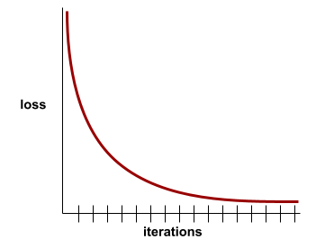
当损失值在每次迭代中的变化非常小或根本没有变化时,即达到收敛状态。例如,以下损失曲线表明模型在大约 700 次迭代时收敛:
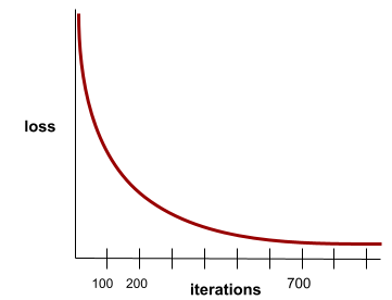
如果继续训练无法改进模型,则表示模型已收敛。
在深度学习中,损失值有时会在许多次迭代中保持不变或几乎不变,然后才会最终下降。如果损失值长时间保持不变,您可能会暂时产生错误的收敛感。
另请参阅早停法。
如需了解详情,请参阅机器学习速成课程中的模型收敛和损失曲线。
对话式编码
您与生成式 AI 模型之间为创建软件而进行的迭代对话。您发出一个描述某种软件的提示。然后,模型会使用该说明生成代码。然后,您发出新的提示来解决之前提示或生成的代码中的缺陷,模型会生成更新后的代码。您和 AI 会不断来回迭代,直到生成的软件足够好为止。
对话编码本质上是氛围编程 (vibe coding)的原始含义。
与规范化编码相对。
凸函数
一种函数,函数图像以上的区域为凸集。典型的凸函数形状类似于字母 U。例如,以下函数均为凸函数:
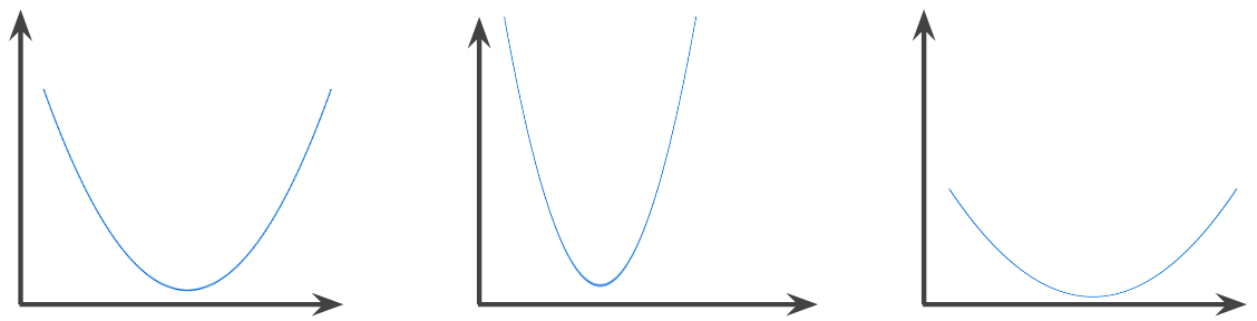
相比之下,以下函数不是凸函数。请注意,图表上方的区域不是凸集:

严格凸函数只有一个局部最小值点,该点也是全局最小值点。经典的 U 形函数是严格凸函数。不过,有些凸函数(例如直线)则不是 U 形函数。
如需了解详情,请参阅机器学习速成课程中的收敛和凸函数。
凸优化
使用梯度下降法等数学技巧来寻找凸函数的最小值。机器学习方面的大量研究都是专注于如何通过公式将各种问题表示成凸优化问题,以及如何更高效地解决这些问题。
如需完整的详细信息,请参阅 Boyd 和 Vandenberghe 合著的 Convex Optimization(《凸优化》)。
凸集
欧氏空间的一个子集,该子集中任意两点之间的连线完全位于该子集中。例如,以下两种形状是凸集:

相比之下,以下两种形状不是凸集:

卷积
在数学中,简单来说,是指两个函数的混合。在机器学习中,卷积结合使用卷积过滤器和输入矩阵来训练权重。
如果没有卷积,机器学习算法就需要学习大张量中每个单元各自的权重。例如,如果机器学习算法在 2K x 2K 的图片上进行训练,则必须找到 400 万个单独的权重。而使用卷积,机器学习算法只需算出卷积过滤器中每个单元的权重,大大减少了训练模型所需的内存。应用卷积过滤器时,只需在各个单元中复制该过滤器,使每个单元都乘以该过滤器。
卷积滤波器
卷积运算中的两个参与方之一。(另一个 actor 是输入矩阵的一个切片。)卷积过滤器是一种矩阵,其秩与输入矩阵相同,但形状小一些。 例如,对于 28x28 的输入矩阵,滤波器可以是任何小于 28x28 的二维矩阵。
在照片处理中,卷积过滤器中的所有单元通常都设置为由 1 和 0 组成的恒定模式。在机器学习中,卷积过滤器通常以随机数作为初始值,然后网络会训练理想值。
卷积层
深度神经网络的一个层,卷积过滤器会在其中传递输入矩阵。以下面的 3x3 卷积过滤器为例:
![一个 3x3 矩阵,包含以下值:[[0,1,0], [1,0,1], [0,1,0]]](https://developers.google.com/static/machine-learning/glossary/images/ConvolutionalFilter33.svg?hl=zh-cn)
以下动画展示了一个卷积层,其中包含 9 个涉及 5x5 输入矩阵的卷积运算。请注意,每个卷积运算都针对输入矩阵的不同 3x3 切片进行运算。生成的 3x3 矩阵(右侧)包含 9 次卷积运算的结果:
![动画:显示两个矩阵。第一个矩阵是 5x5 矩阵:[[128,97,53,201,198], [35,22,25,200,195],
[37,24,28,197,182], [33,28,92,195,179], [31,40,100,192,177]]。
第二个矩阵是 3x3 矩阵:
[[181,303,618], [115,338,605], [169,351,560]]。
第二个矩阵是通过对 5x5 矩阵的不同 3x3 子集应用卷积滤波器 [[0, 1, 0], [1, 0, 1], [0, 1, 0]] 计算得出的。](https://developers.google.com/static/machine-learning/glossary/images/AnimatedConvolution.gif?hl=zh-cn)
卷积神经网络
一种神经网络,其中至少有一层为卷积层。典型的卷积神经网络由以下层的某种组合构成:
卷积神经网络在某些类型的问题(例如图像识别)中取得了巨大成功。
卷积运算
如下所示的两步数学运算:
- 对卷积过滤器和输入矩阵切片执行元素级乘法。(输入矩阵切片与卷积过滤器具有相同的秩和大小。)
- 对生成的积矩阵中的所有值求和。
例如,考虑以下 5x5 输入矩阵:
![5x5 矩阵:[[128,97,53,201,198], [35,22,25,200,195],
[37,24,28,197,182], [33,28,92,195,179], [31,40,100,192,177]]。](https://developers.google.com/static/machine-learning/glossary/images/ConvolutionalLayerInputMatrix.svg?hl=zh-cn)
现在,假设有以下 2x2 卷积过滤器:
![2x2 矩阵:[[1, 0], [0, 1]]](https://developers.google.com/static/machine-learning/glossary/images/ConvolutionalLayerFilter.svg?hl=zh-cn)
每个卷积运算都涉及输入矩阵的单个 2x2 切片。例如,假设我们使用输入矩阵左上角的 2x2 切片。因此,此切片的卷积运算如下所示:
![将卷积过滤器 [[1, 0], [0, 1]] 应用于输入矩阵的左上角 2x2 部分,即 [[128,97], [35,22]]。卷积滤波器会使 128 和 22 保持不变,但会将 97 和 35 归零。因此,卷积运算会产生值 150 (128+22)。](https://developers.google.com/static/machine-learning/glossary/images/ConvolutionalLayerOperation.svg?hl=zh-cn)
卷积层由一系列卷积运算组成,每个卷积运算都针对不同的输入矩阵切片。
COPA
选择合理替代方案的缩写。
费用
与损失的含义相同。
共同训练
一种半监督式学习方法,在满足以下所有条件时特别有用:
共同训练本质上是将独立信号放大为更强的信号。 例如,假设有一个分类模型,用于将每辆二手车归类为好或坏。一组预测性特征可能侧重于汽车的年份、品牌和型号等汇总特征;另一组预测性特征可能侧重于前车主的驾驶记录和汽车的保养历史记录。
关于协同训练的开创性论文是 Blum 和 Mitchell 撰写的将带标签的数据和不带标签的数据与协同训练相结合。
反事实公平性
一种公平性指标,用于检查分类模型是否会针对以下两种个体生成相同的结果:一种个体与另一种个体完全相同,只是在一种或多种敏感属性方面有所不同。评估分类模型的反事实公平性是发现模型中潜在偏差来源的一种方法。
如需了解详情,请参阅以下任一内容:
- 公平性:反事实公平性(机器学习速成课程)。
- 当世界相撞时:在公平性中整合不同的反事实假设
覆盖偏差
请参阅选择性偏差。
歧义
含义不明确的句子或词组。 歧义是自然语言理解的一个重大问题。例如,标题“Red Tape Holds Up Skyscraper”存在歧义,因为 NLU 模型可能会从字面解读该标题,也可能会从象征角度进行解读。
评论者
与 Deep Q-Network 的含义相同。
交叉熵
对数损失函数到多类别分类问题的泛化。交叉熵可以量化两种概率分布之间的差异。另请参阅困惑度。
交叉验证
一种机制,使用从训练集中保留的一个或多个不重叠的数据子集测试模型,以估计该模型泛化到新数据的效果。
累积分布函数 (CDF)
一种用于定义小于或等于目标值的样本频率的函数。例如,假设存在一个连续值的正态分布。CDF 会告诉您,大约 50% 的样本应小于或等于平均值,大约 84% 的样本应小于或等于平均值加一个标准差。
D
数据分析
根据样本、测量结果和可视化内容理解数据。数据分析在首次收到数据集时且构建第一个模型之前特别有用。此外,数据分析在理解实验和调试系统问题方面也至关重要。
数据增强
通过转换现有样本来创建其他样本,人为地增加训练样本的范围和数量。例如,假设图像是其中一个特征,但数据集包含的图像样本不足以供模型学习有用的关联。 理想情况下,您需要向数据集添加足够的有标签图像,才能使模型正常训练。如果不可行,则可以通过数据增强旋转、拉伸和翻转每张图像,以生成原始照片的多个变体,这样可能会生成足够的有标签数据来实现很好的训练效果。
DataFrame
一种热门的 pandas 数据类型,用于表示内存中的数据集。
DataFrame 类似于表格或电子表格。DataFrame 的每一列都有一个名称(标题),每一行都由一个唯一编号标识。
DataFrame 中的每一列都以二维数组的形式构建,但每一列都可以分配自己的数据类型。
另请参阅官方 pandas.DataFrame 参考页面。
数据并行处理
一种可扩展训练或推理的方式,可将整个模型复制到多个设备上,然后将输入数据的一个子集传递给每个设备。数据并行处理可支持针对非常大的批次大小进行训练和推理;不过,数据并行处理要求模型足够小,以适应所有设备。
数据并行处理通常可加快训练和推理速度。
另请参阅模型并行性。
Dataset API (tf.data)
一种高阶 TensorFlow API,用于读取数据并将其转换为机器学习算法所需的格式。tf.data.Dataset 对象表示一系列元素,其中每个元素都包含一个或多个张量。tf.data.Iterator 对象可用于访问 Dataset 的元素。
数据集(data set 或 dataset)
原始数据的集合,通常(但不一定)以以下格式之一进行整理:
- 电子表格
- 采用 CSV(逗号分隔值)格式的文件
决策边界
模型在二元分类或多类别分类问题中学习到的类别之间的分隔符。例如,在以下表示某个二元分类问题的图片中,决策边界是橙色类别和蓝色类别之间的分界线:

决策森林
一种由多个决策树创建的模型。决策森林通过汇总其决策树的预测结果来进行预测。常见的决策森林类型包括随机森林和梯度提升树。
如需了解详情,请参阅决策森林课程中的决策森林部分。
决策阈值
与分类阈值的含义相同。
决策树
一种监督学习模型,由一组按层次结构组织的条件和叶组成。例如,以下是一个决策树:
解码器
一般来说,任何将经过处理的密集型内部表示形式转换为更原始的稀疏型外部表示形式的机器学习系统。
解码器通常是较大模型的组成部分,并且经常与编码器配对使用。
在序列到序列任务中,解码器从编码器生成的内部状态开始预测下一个序列。
如需了解 Transformer 架构中解码器的定义,请参阅 Transformer。
如需了解详情,请参阅机器学习速成课程中的大型语言模型。
深度模型
深度模型也称为深度神经网络。
与宽度模型相对。
一种非常流行的深度神经网络
与深度模型的含义相同。
深度 Q 网络 (DQN)
在 Q-learning 中,深度神经网络会预测 Q 函数。
评判家是深度 Q 网络的同义词。
人口统计均等
一种公平性指标,如果模型分类的结果不依赖于给定的敏感属性,则满足该指标。
例如,如果小人国人和巨人国人都申请了 Glubbdubdrib 大学,那么如果录取的小人国人百分比与录取的大人国人百分比相同,则实现了人口统计学上的平等,无论一个群体是否比另一个群体平均而言更符合条件。
与均衡赔率和机会均等形成对比,后者允许分类结果总体上取决于敏感属性,但不允许某些指定标准答案标签的分类结果取决于敏感属性。如需查看直观图表,了解在优化人口统计学均等性时需要做出的权衡,请参阅“通过更智能的机器学习避免歧视”。
如需了解详情,请参阅机器学习速成课程中的公平性:人口统计学奇偶性。
降噪
一种常见的自监督式学习方法,其中:
去噪功能可实现从无标签示例中学习。 原始数据集用作目标或标签,而噪声数据用作输入。
部分掩码语言模型使用以下去噪方式:
- 通过屏蔽部分令牌,人为地向无标签句子添加噪声。
- 模型会尝试预测原始 token。
密集特征
一种特征,其中大多数或所有值都不为零,通常是浮点值的 Tensor。例如,以下 10 元素张量是密集张量,因为其中 9 个值不为零:
| 8 | 3 | 7 | 5 | 2 | 4 | 0 | 4 | 9 | 6 |
与稀疏特征相对。
密集层
与全连接层的含义相同。
深度
神经网络中以下各项的总和:
例如,具有 5 个隐藏层和 1 个输出层的神经网络的深度为 6。
请注意,输入层不会影响深度。
深度可分离卷积神经网络 (sepCNN)
基于 Inception 的卷积神经网络架构,但其中的 Inception 模块被替换为深度可分离卷积。也称为 Xception。
深度可分离卷积(也简称为可分离卷积)将标准 3D 卷积分解为两个单独的卷积运算,这两个运算在计算上更高效:首先是深度为 1 (n ✕ n ✕ 1) 的深度卷积,然后是长度和宽度为 1 (1 ✕ 1 ✕ n) 的点状卷积。
如需了解详情,请参阅 Xception:使用深度可分离卷积的深度学习。
派生标签
与代理标签的含义相同。
确定性
一种针对给定输入始终返回相同输出的系统。例如,ReLU 函数是确定性函数,因为:
- 当输入为负数时,输出始终为 0。
- 当输入为非负数时,输出始终等于输入。
相比之下,每次调用时都返回随机数的函数是不确定性的。
确定性系统通常比非确定性系统更容易测试。
LLM 通常是非确定性的;也就是说,LLM 对同一提示的回答往往不同。
设备
一个多含义术语,具有以下两种可能的定义:
- 一类可运行 TensorFlow 会话的硬件,包括 CPU、GPU 和 TPU。
- 在 加速器芯片(GPU 或 TPU)上训练机器学习模型时,实际操控张量和嵌入的系统部分。 设备在加速器芯片上运行。相比之下,宿主通常在 CPU 上运行。
差分隐私
在机器学习中,一种用于保护模型训练集中包含的任何敏感数据(例如个人信息)免遭泄露的匿名化方法。这种方法可确保模型不会学习或记住有关特定个人的太多信息。为此,我们在模型训练期间进行抽样并添加噪声,以模糊单个数据点,从而降低泄露敏感训练数据的风险。
差分隐私也用于机器学习之外的领域。例如,数据科学家有时会在计算不同人口统计特征的产品使用情况统计信息时使用差分隐私来保护个人隐私。
降维
减少用于表示特征向量中特定特征的维度的数量,通常通过转换为嵌入向量来实现此操作。
维度
一个具有多重含义的术语,包括以下含义:
Tensor中的坐标级别数量。例如:
- 标量有零个维度,例如
["Hello"]。 - 向量有一个维度,例如
[3, 5, 7, 11]。 - 矩阵有两个维度,例如
[[2, 4, 18], [5, 7, 14]]。 您可以使用一个坐标唯一指定一维向量中的特定单元;您需要使用两个坐标唯一指定二维矩阵中的特定单元。
- 标量有零个维度,例如
特征向量中的条目数。
嵌入层中的元素数。
直接提示
与零样本提示的含义相同。
离散特征
一种特征,包含有限个可能值。例如,值可能仅为 animal、vegetable 或 mineral 的特征是离散(或分类)特征。
与连续特征相对。
判别模型
一种通过一个或多个特征组成的集合预测标签的模型。更正式地讲,判别模型会根据特征和权重定义输出的条件概率;即:
p(output | features, weights)
例如,如果一个模型要通过特征和权重预测某封电子邮件是否是垃圾邮件,那么该模型为判别模型。
绝大多数监督学习模型(包括分类模型和回归模型)都是判别模型。
与生成模型相对。
判别器
一种确定样本是否真实的系统。
或者,生成对抗网络中的子系统,用于确定生成器创建的样本是真实的还是虚假的。
如需了解详情,请参阅 GAN 课程中的判别器。
不同影响
做出有关人员的决策,但这些决策对不同的人口子群组的影响不成比例。这通常是指算法决策流程对某些子群组的伤害或益处大于其他子群组的情况。
例如,假设某个算法用于确定小人国居民是否符合微型住宅贷款的申请条件,如果申请人的邮寄地址包含某个邮政编码,该算法更有可能将申请人归类为“不符合条件”。如果大端序小人国居民比小端序小人国居民更可能拥有此邮政编码的邮寄地址,那么此算法可能会造成差别影响。
与差别对待形成对比,后者侧重于当子群组特征是算法决策过程的显式输入时导致的不公平现象。
差别待遇
在算法决策过程中纳入受试者的敏感属性,以便区别对待不同的人群子群组。
例如,假设有一种算法,可根据小人国居民在贷款申请中提供的数据来确定他们是否符合微型住宅贷款的条件。如果算法使用 Lilliputian 的从属关系(即大端序或小端序)作为输入,则会在该维度上实施差别对待。
与差异化影响形成对比,后者侧重于算法决策对子群体的社会影响方面的差异,无论这些子群体是否是模型的输入。
蒸馏
将一个模型(称为教师)的大小缩减为较小的模型(称为学生)的过程,该较小的模型尽可能忠实地模拟原始模型的预测结果。知识蒸馏之所以有用,是因为较小的模型比较大的模型(教师模型)具有以下两个主要优势:
- 推理时间更短
- 减少了内存和能耗用量
不过,学生的预测通常不如教师的预测。
蒸馏训练学生模型,以最大限度地减少基于学生模型和教师模型预测输出之间差异的损失函数。
比较和对比蒸馏与以下术语:
如需了解详情,请参阅机器学习速成课程中的 LLM:微调、蒸馏和提示工程。
分布式训练
给定特征或标签的不同值的频次和范围。分布可反映特定值的可能性。
下图显示了两种不同分布的直方图:
- 左侧:财富与拥有相应财富的人数之间的幂律分布。
- 右侧是身高与拥有相应身高的人数之间的正态分布。
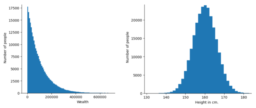
了解每个特征和标签的分布情况有助于您确定如何归一化值和检测离群值。
分布外是指未出现在数据集中的值或非常罕见的值。例如,对于由猫图片组成的数据集,土星的图片会被视为分布外数据。
分裂式层次聚类
请参阅层次聚类。
降采样
一个多含义术语,可以理解为下列两种含义之一:
- 减少特征中的信息量,以便更有效地训练模型。例如,在训练图像识别模型之前,将高分辨率图像降采样为分辨率较低的格式。
- 使用占比异常低、得到过度代表的类别样本训练模型,以改进未得到充分代表的类别的模型训练效果。 例如,在类别不平衡的数据集中,模型往往会学习到很多关于多数类的知识,但关于少数类的知识却不够。降采样有助于平衡多数类和少数类的训练量。
如需了解详情,请参阅机器学习速成课程中的数据集:不平衡的数据集。
DQN
深度 Q 网络的缩写。
dropout 正规化
一种正则化形式,在训练神经网络时非常有用。Dropout 正规化的运作机制是,在一个梯度步中移除从神经网络层中随机选择的固定数量的单元。丢弃的单元越多,正则化就越强。这类似于训练神经网络以模拟较小网络的指数级规模集成。如需完整的详细信息,请参阅 Dropout: A Simple Way to Prevent Neural Networks from Overfitting(《Dropout:一种防止神经网络过拟合的简单方法》)。
动态
经常或持续做的事情。 在机器学习中,“动态”和“在线”是同义词。以下是机器学习中动态和在线的常见用途:
- 动态模型(或在线模型)是一种经常或持续重新训练的模型。
- 动态训练(或在线训练)是指频繁或持续的训练过程。
- 动态推理(或在线推理)是指根据需要生成预测的过程。
动态模型
一种经常(甚至持续)重新训练的模型。动态模型是“终身学习者”,会不断适应不断变化的数据。动态模型也称为在线模型。
与静态模型相对。
E
即刻执行
一种 TensorFlow 编程环境,操作可在其中立即运行。相比之下,在图执行中调用的操作在得到明确评估之前不会运行。即刻执行是一种命令式接口,就像大多数编程语言中的代码一样。相比图执行程序,调试即刻执行程序通常要容易得多。
早停法
一种正则化方法,涉及在训练损失停止下降之前结束训练。在早停法中,当验证数据集的损失开始增加时(即泛化性能变差时),您会故意停止训练模型。
与提前退出相对。
推土机距离 (EMD)
一种衡量两种分布相对相似度的指标。 推土机距离越小,分布越相似。
编辑距离
衡量两个文本字符串彼此之间的相似程度。在机器学习中,编辑距离非常有用,原因如下:
- 编辑距离很容易计算。
- 编辑距离可以比较已知彼此相似的两个字符串。
- 编辑距离可以确定不同字符串与给定字符串的相似程度。
编辑距离有多种定义,每种定义都使用不同的字符串操作。如需查看示例,请参阅 Levenshtein 距离。
Einsum 表示法
一种用于描述如何组合两个张量的有效表示法。张量的组合方式是将一个张量的元素与另一个张量的元素相乘,然后将乘积相加。 Einsum 表示法使用符号来标识每个张量的轴,并重新排列这些相同的符号来指定新生成的张量的形状。
NumPy 提供了一个通用的 Einsum 实现。
嵌入层
一种特殊的隐藏层,可针对高维分类特征进行训练,以逐步学习低维嵌入向量。与仅基于高维分类特征进行训练相比,嵌入层可让神经网络的训练效率大幅提高。
例如,地球目前支持约 73,000 种树。假设树种是模型中的一个特征,那么模型的输入层将包含一个长度为 73,000 的独热向量。
例如,baobab 可能会以如下方式表示:
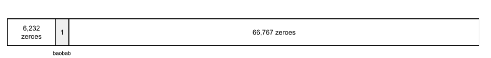
包含 73,000 个元素的数组非常长。如果您不向模型添加嵌入层,则由于要乘以 72,999 个零,训练将非常耗时。假设您选择的嵌入层包含 12 个维度。因此,嵌入层将逐渐学习每种树木的新嵌入向量。
在某些情况下,哈希处理是嵌入层的合理替代方案。
如需了解详情,请参阅机器学习速成课程中的嵌入。
嵌入空间
更高维度的向量空间中的特征所映射到的 d 维向量空间。嵌入空间经过训练,可捕获对预期应用有意义的结构。
嵌入向量
广义上讲,是指从任何 隐藏层提取的浮点数数组,用于描述该隐藏层的输入。 通常,嵌入向量是在嵌入层中训练的浮点数数组。例如,假设嵌入层必须学习地球上 73,000 种树木中每种树木的嵌入向量。以下数组可能就是一棵猴面包树的嵌入向量:
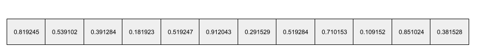
嵌入向量不是一堆随机数字。嵌入层通过训练来确定这些值,类似于神经网络在训练期间学习其他权重的方式。数组的每个元素都是树种在某个特征方面的评级。哪个元素代表哪种树种的特征?人类很难确定这一点。
嵌入向量在数学上令人称奇之处在于,相似的内容具有相似的浮点数集。例如,相似的树种比不相似的树种具有更相似的浮点数集。红杉和巨杉是相关的树种,因此它们将具有比红杉和椰子树更相似的一组浮点数。即使您使用相同的输入重新训练模型,嵌入向量中的数字也会在每次重新训练模型时发生变化。
突现行为
LLM 针对未明确训练过的提示生成回答的能力。
经验累积分布函数(eCDF 或 EDF)
基于真实数据集的实证测量结果的累积分布函数。沿 x 轴上任意点的函数值是数据集中小于或等于指定值的观测值的比例。
经验风险最小化 (ERM)
选择可最大限度减少训练集损失的函数。与结构风险最小化相对。
编码器
一般来说,任何将原始、稀疏或外部表示形式转换为经过更多处理、更密集或更内部的表示形式的机器学习系统。
编码器通常是较大模型的组成部分,并且经常与解码器配对使用。有些 Transformer 会将编码器与解码器配对,不过其他 Transformer 只使用编码器或只使用解码器。
有些系统使用编码器的输出作为分类或回归网络的输入。
在序列到序列任务中,编码器会接收输入序列并返回内部状态(一个向量)。然后,解码器使用该内部状态来预测下一个序列。
如需了解 Transformer 架构中编码器的定义,请参阅 Transformer。
如需了解详情,请参阅机器学习速成课程中的大语言模型:什么是大语言模型。
endpoints
可通过网络寻址的位置(通常为网址),服务可通过该位置访问。
集成学习
一组独立训练的模型,其预测结果经过平均处理或汇总。在许多情况下,集成模型比单个模型能做出更好的预测。例如,随机森林是由多个决策树构建的集成学习模型。请注意,并非所有决策森林都是集成学习模型。
如需了解详情,请参阅机器学习速成课程中的随机森林。
熵
在 信息论中,用于描述概率分布的不可预测程度。或者,熵也可以定义为每个示例包含的信息量。当随机变量的所有值具有相同的可能性时,分布的熵最大。
具有两个可能值“0”和“1”(例如,二元分类问题中的标签)的集合的熵具有以下公式:
H = -p log p - q log q = -p log p - (1-p) * log (1-p)
其中:
- H 是熵。
- p 是“1”示例的比例。
- q 是“0”示例的比例。请注意,q = (1 - p)
- 对数通常为以 2 为底的对数。在本例中,熵单位为比特。
例如,假设情况如下:
- 100 个示例包含值“1”
- 300 个示例包含值“0”
因此,熵值为:
- p = 0.25
- q = 0.75
- H = (-0.25)log2(0.25) - (0.75)log2(0.75) = 每个示例 0.81 位
完全平衡的集合(例如,200 个“0”和 200 个“1”)的每个示例的熵为 1.0 位。随着集合变得越来越不平衡,其熵会趋向于 0.0。
在决策树中,熵有助于制定信息增益,从而帮助分裂器在分类决策树的增长过程中选择条件。
将熵与以下对象进行比较:
熵通常称为“香农熵”。
如需了解详情,请参阅决策森林课程中的使用数值特征进行二元分类的精确分裂器。
环境
在强化学习中,包含智能体并允许智能体观察世界状态的世界。例如,所表示的世界可以是国际象棋等游戏,也可以是迷宫等现实世界。当智能体对环境应用某项操作时,环境会在状态之间转换。
环境接地
在智能体循环的反馈阶段,流回智能体的原始数据。例如,代理的环境接地可能包括错误日志或新创建的网页的 HTML。
分集
情景记忆
在 LLM 中,指训练后学到的信息。相比之下,语义记忆是在训练期间学习的信息。情景记忆可以是临时的(例如,仅在当前聊天机器人会话中持续存在),也可以是更持久的(例如,在用户调用的每个会话中持续存在)。
另请参阅程序性记忆。
周期数
在训练时,对整个训练集的一次完整遍历,不会漏掉任何一个样本。
一个周期表示 N/批次大小次训练迭代,其中 N 是样本总数。
例如,假设存在以下情况:
- 该数据集包含 1,000 个示例。
- 批次大小为 50 个样本。
因此,一个周期需要 20 次迭代:
1 epoch = (N/batch size) = (1,000 / 50) = 20 iterations
如需了解详情,请参阅机器学习速成课程中的线性回归:超参数。
epsilon-greedy 策略
在强化学习中,一种政策,以 epsilon 概率遵循随机政策,否则遵循贪婪政策。例如,如果 epsilon 为 0.9,则政策有 90% 的时间遵循随机政策,有 10% 的时间遵循贪婪政策。
在连续的剧集中,算法会减小 epsilon 的值,以便从遵循随机政策转为遵循贪婪政策。通过调整政策,智能体首先会随机探索环境,然后贪婪地利用随机探索的结果。
机会均等
一种公平性指标,用于评估模型是否能针对敏感属性的所有值同样准确地预测出理想结果。换句话说,如果模型的理想结果是正类别,那么目标就是让所有组的真正例率保持一致。
机会平等与赔率均衡有关,后者要求所有群组的真正例率和假正例率都相同。
假设 Glubbdubdrib 大学允许小人国人和巨人国人参加严格的数学课程。Lilliputians 的中学提供完善的数学课程,绝大多数学生都符合大学课程的入学条件。Brobdingnagian 的中学根本不提供数学课程,因此,他们的学生中只有极少数人符合条件。如果合格学生被录取的机会均等,无论他们是小人国人还是巨人国人,那么对于“录取”这一首选标签,机会均等就满足了。
例如,假设有 100 名小人国人和 100 名巨人国人申请了 Glubbdubdrib 大学,录取决定如下:
表 1. Lilliputian 申请者(90% 符合条件)
| 符合资格 | 不合格 | |
|---|---|---|
| 已允许 | 45 | 3 |
| 已拒绝 | 45 | 7 |
| 总计 | 90 | 10 |
|
被录取的合格学生所占百分比:45/90 = 50% 被拒的不合格学生所占百分比:7/10 = 70% 被录取的小人国学生所占总百分比:(45+3)/100 = 48% |
||
表 2. Brobdingnagian 申请者(10% 符合条件):
| 符合资格 | 不合格 | |
|---|---|---|
| 已允许 | 5 | 9 |
| 已拒绝 | 5 | 81 |
| 总计 | 10 | 90 |
|
符合条件的学生录取百分比:5/10 = 50% 不符合条件的学生拒绝百分比:81/90 = 90% Brobdingnagian 学生总录取百分比:(5+9)/100 = 14% |
||
上述示例满足了合格学生在入学方面的机会平等,因为合格的利立浦特人和布罗卜丁奈格人都只有 50% 的入学机会。
虽然满足了机会均等,但未满足以下两个公平性指标:
- 人口同等性:小人国人和巨人国人被大学录取的机会不同;48% 的小人国学生被录取,但只有 14% 的巨人国学生被录取。
- 机会均等:虽然符合条件的小人国学生和巨人国学生被录取的几率相同,但不符合条件的小人国学生和巨人国学生被拒绝的几率相同这一额外限制条件并未得到满足。不合格的 Lilliputian 的拒绝率为 70%,而不合格的 Brobdingnagian 的拒绝率为 90%。
如需了解详情,请参阅机器学习速成课程中的公平性:机会平等。
均衡赔率
一种公平性指标,用于评估模型是否能针对敏感属性的所有值,同样准确地预测正类别和负类别的结果,而不仅仅是其中一个类别。换句话说,所有组的真正例率和假负例率都应相同。
均衡赔率与机会均等相关,后者仅关注单个类别(正类别或负类别)的错误率。
例如,假设 Glubbdubdrib 大学允许小人国人和巨人国人同时参加一项严格的数学课程。Lilliputians 的中学提供全面的数学课程,绝大多数学生都符合大学课程的入学条件。Brobdingnagians 的中学根本不提供数学课程,因此,他们的学生中只有极少数人符合条件。只要满足以下条件,即可实现均衡赔率:无论申请者是小人国人还是巨人国人,如果他们符合条件,被该计划录取的可能性都相同;如果他们不符合条件,被拒绝的可能性也相同。
假设有 100 名小人国人和 100 名巨人国人申请了 Glubbdubdrib 大学,录取决定如下:
表 3. Lilliputian 申请者(90% 符合条件)
| 符合资格 | 不合格 | |
|---|---|---|
| 已允许 | 45 | 2 |
| 已拒绝 | 45 | 8 |
| 总计 | 90 | 10 |
|
被录取的合格学生所占百分比:45/90 = 50% 被拒绝的不合格学生所占百分比:8/10 = 80% 被录取的 Lilliputian 学生总数所占百分比:(45+2)/100 = 47% |
||
表 4. Brobdingnagian 申请者(10% 符合条件):
| 符合资格 | 不合格 | |
|---|---|---|
| 已允许 | 5 | 18 |
| 已拒绝 | 5 | 72 |
| 总计 | 10 | 90 |
|
符合条件的学生录取百分比:5/10 = 50% 不符合条件的学生拒绝百分比:72/90 = 80% Brobdingnagian 学生总录取百分比:(5+18)/100 = 23% |
||
由于符合条件的小人国学生和巨人国学生被录取的概率均为 50%,而不符合条件的小人国学生和巨人国学生被拒绝的概率均为 80%,因此等几率条件得以满足。
“监督学习中的机会平等”中对均衡赔率的正式定义如下:“如果预测器 Ŷ 和受保护属性 A 在以 Y 为条件的情况下相互独立,则预测器 Ŷ 满足关于受保护属性 A 和结果 Y 的均衡赔率。”
Estimator
已弃用的 TensorFlow API。使用 tf.keras 而不是 Estimator。
evals
主要用作 LLM 评估的缩写。 更广泛地说,evals 是任何形式的评估的缩写。
评估
衡量模型质量或比较不同模型的过程。
若要评估监督式机器学习模型,您通常需要根据验证集和测试集来判断模型的效果。评估 LLM 通常涉及更广泛的质量和安全性评估。
评估器代理
在结果最终确定之前评估其他代理的结果的代理。您可以将一个代理想象成制造产品的代理,而将另一个代理(评估代理)想象成在产品发布之前测试该产品的代理。
评价者是评估者代理的同义词。
完全匹配
一种非此即彼的指标,即模型的输出要么与标准答案或参考文本完全一致,要么完全不一致。例如,如果标准答案是 orange,则只有模型输出 orange 满足完全匹配条件。
完全匹配还可以评估输出为序列(已排名商品列表)的模型。一般来说,完全匹配要求生成的排名列表与标准答案完全一致;也就是说,两个列表中的每个项目都必须按相同的顺序排列。不过,如果评估依据包含多个正确序列,那么完全匹配仅要求模型的输出与一个正确序列匹配。
示例
一行特征的值,可能还包含一个标签。监督学习中的示例大致分为两类:
例如,假设您正在训练一个模型,以确定天气条件对学生考试成绩的影响。以下是三个带标签的示例:
| 功能 | 标签 | ||
|---|---|---|---|
| 温度 | 湿度 | 压力 | 测试分数 |
| 15 | 47 | 998 | 良好 |
| 19 | 34 | 1020 | 极佳 |
| 18 | 92 | 1012 | 差 |
以下是三个未标记的示例:
| 温度 | 湿度 | 压力 | |
|---|---|---|---|
| 12 | 62 | 1014 | |
| 21 | 47 | 1017 | |
| 19 | 41 | 1021 |
数据集的行通常是示例的原始来源。 也就是说,一个示例通常由数据集中的一部分列组成。此外,示例中的特征还可以包括合成特征,例如特征交叉。
如需了解详情,请参阅“机器学习简介”课程中的监督式学习。
经验回放
在强化学习中,一种用于减少训练数据中时间相关性的 DQN 技术。代理将状态转换存储在回放缓冲区中,然后从回放缓冲区中抽样转换以创建训练数据。
实验者偏差
请参阅确认偏差。
梯度爆炸问题
深度神经网络(尤其是循环神经网络)中的梯度出人意料地变得陡峭(高)的趋势。陡峭的梯度通常会导致深度神经网络中每个节点的权重发生非常大的更新。
如果模型出现梯度爆炸问题,则很难或无法进行训练。梯度裁剪可以缓解此问题。
与梯度消失问题相对。
极速摘要 (xsum)
用于评估 LLM 总结单个文档的能力的数据集。 数据集中的每个条目都包含以下内容:
- 由英国广播公司 (BBC) 撰写的一份文档。
- 相应文档的单句摘要。
如需了解详情,请参阅不要给我详细信息,只要摘要!Topic-Aware Convolutional Neural Networks for Extreme Summarization。
F
F1
一种“总览”二元分类指标,同时依赖于精确率和召回率。公式如下:
真实性
在机器学习领域中,一种描述模型的属性,该模型的输出基于现实。事实性是一个概念,而不是一个指标。例如,假设您向大语言模型发送以下提示:
食盐的化学式是什么?
如果模型侧重于事实性,则会回答:
NaCl
人们很容易认为所有模型都应基于事实。不过,某些提示(例如以下提示)应促使生成式 AI 模型优化创意性,而不是事实性。
给我讲一个关于宇航员和毛毛虫的五行打油诗。
这样创作出的五行打油诗不太可能基于现实。
与事实依据相对。
公平性约束
对算法应用限制条件,以确保满足一项或多项公平性定义。公平性限制的示例包括:- 对模型输出进行后处理。
- 更改损失函数,以纳入对违反公平性指标的行为的惩罚。
- 直接向优化问题添加数学约束。
公平性指标
可衡量的“公平性”的数学定义。 一些常用的公平性指标包括:
许多公平性指标是互斥的;请参阅公平性指标互不相容。
假负例 (FN)
被模型错误地预测为负类别的样本。例如,模型预测某封电子邮件不是垃圾邮件(负类别),但该电子邮件实际上是垃圾邮件。
假负例率
模型错误地将实际正例预测为负类别 的比例。以下公式用于计算假负率:
如需了解详情,请参阅机器学习速成课程中的阈值和混淆矩阵。
假正例 (FP)
被模型错误地预测为正类别的样本。例如,模型预测某封电子邮件是垃圾邮件(正类别),但该电子邮件实际上不是垃圾邮件。
如需了解详情,请参阅机器学习速成课程中的阈值和混淆矩阵。
假正例率 (FPR)
模型错误地将实际负例预测为正类别。以下公式用于计算假正例率:
假正例率是 ROC 曲线的 x 轴。
如需了解详情,请参阅机器学习速成课程中的分类:ROC 和 AUC。
快速衰减
一种用于提升 大语言模型 性能的训练技术。快速衰减是指在训练期间快速降低学习速率。此策略有助于防止模型对训练数据出现过拟合,并提高泛化能力。
功能
机器学习模型的输入变量。一个示例包含一个或多个特征。例如,假设您正在训练一个模型,以确定天气条件对学生考试成绩的影响。下表显示了三个示例,每个示例都包含三个特征和一个标签:
| 功能 | 标签 | ||
|---|---|---|---|
| 温度 | 湿度 | 压力 | 测试分数 |
| 15 | 47 | 998 | 92 |
| 19 | 34 | 1020 | 84 |
| 18 | 92 | 1012 | 87 |
与标签相对。
如需了解详情,请参阅“机器学习简介”课程中的监督式学习。
特征组合
例如,假设有一个“情绪预测”模型,它使用以下四个区间之一来表示温度:
freezingchillytemperatewarm
并以以下三个区间之一表示风速:
stilllightwindy
如果不进行特征交叉,线性模型会针对上述七个不同的分桶分别进行独立训练。因此,模型会基于 freezing 进行训练,而不会基于 windy 进行训练。
或者,您也可以创建温度和风速的特征组合。此合成特征将具有以下 12 个可能的值:
freezing-stillfreezing-lightfreezing-windychilly-stillchilly-lightchilly-windytemperate-stilltemperate-lighttemperate-windywarm-stillwarm-lightwarm-windy
借助特征交叉,模型可以了解freezing-windy天和freezing-still天之间的情绪差异。
如果您使用两个各自具有许多不同分箱的合成特征创建特征,则生成的特征组合将具有大量可能的组合。例如,如果一个特征有 1,000 个分桶,另一个特征有 2,000 个分桶,那么生成的特征组合将有 2,000,000 个分桶。
从形式上讲,交叉联接是笛卡尔积。
特征交叉主要用于线性模型,很少用于神经网络。
如需了解详情,请参阅机器学习速成课程中的分类数据:特征组合。
特征工程
一种流程,包括以下步骤:
- 确定哪些特征可能在训练模型方面非常有用。
- 将数据集中的原始数据转换为这些特征的高效版本。
例如,您可能会认为 temperature 是一项有用的功能。然后,您可以尝试使用分桶来优化模型可从不同 temperature 范围中学习的内容。
如需了解详情,请参阅机器学习速成课程中的数值数据:模型如何使用特征向量提取数据。
特征提取
一个多含义术语,具有下列两种含义之一:
特征重要性
与变量重要性的含义相同。
特征集
机器学习模型训练时采用的一组特征。 例如,用于预测房价的模型的简单特征集可能包含邮政编码、房产面积和房产状况。
特征规范
介绍从 tf.Example 协议缓冲区提取特征数据所需的信息。由于 tf.Example 协议缓冲区只是一个数据容器,因此您必须指定以下内容:
- 要提取的数据(即特征的键)
- 数据类型(例如,float 或 int)
- 长度(固定或可变)
特征向量
构成示例的特征值数组。特征向量在训练和推理期间作为输入。例如,具有两个离散特征的模型的特征向量可能如下所示:
[0.92, 0.56]

每个示例都为特征向量提供不同的值,因此下一个示例的特征向量可能如下所示:
[0.73, 0.49]
特征工程决定了如何在特征向量中表示特征。例如,具有 5 个可能值的二元分类特征可以使用独热编码来表示。在这种情况下,特定示例的特征向量部分将包含四个零和一个位于第三位置的 1.0,如下所示:
[0.0, 0.0, 1.0, 0.0, 0.0]
再举一个例子,假设您的模型包含三个特征:
- 采用独热编码表示的具有五个可能值的二元分类特征;例如:
[0.0, 1.0, 0.0, 0.0, 0.0] - 另一个二元分类特征,具有 3 个可能的值,以独热编码表示;例如:
[0.0, 0.0, 1.0] - 浮点特征;例如:
8.3。
在这种情况下,每个示例的特征向量将由 9 个值表示。根据上一个列表中的示例值,特征向量将为:
0.0
1.0
0.0
0.0
0.0
0.0
0.0
1.0
8.3
如需了解详情,请参阅机器学习速成课程中的数值数据:模型如何使用特征向量提取数据。
特征化
从文档或视频等输入源中提取特征并将这些特征映射到特征向量的过程。
一些机器学习专家将“featurization”用作特征工程或特征提取的同义词。
联合学习
是一种分布式机器学习方法,使用驻留在智能手机等设备上的分散样本来训练机器学习模型。在联邦学习中,一部分设备会从中央协调服务器下载当前模型。设备会使用存储在设备上的示例来改进模型。然后,设备会将模型改进(但不会上传训练示例)上传到协调服务器,在服务器上,这些改进会与其他更新聚合,从而生成改进的全局模型。聚合完成后,设备计算出的模型更新不再需要,可以舍弃。
由于训练示例永远不会上传,因此联邦学习遵循聚焦数据收集和数据最小化的隐私原则。
如需了解详情,请参阅联邦学习漫画(没错,就是漫画)。
反馈
智能体循环中的一个阶段,在此阶段,智能体会评估在行动阶段采取的行动。例如,如果代理在行动阶段发送了 API 请求,反馈阶段可能会确定 API 响应是否成功。
反馈环
在机器学习中,一种模型预测会影响同一模型或其他模型的训练数据的情况。例如,推荐电影的模型会影响用户看到的电影,进而影响后续的电影推荐模型。
如需了解详情,请参阅机器学习速成课程中的生产环境中的机器学习系统:需要提出的问题。
前馈神经网络 (FFN)
没有循环或递归连接的神经网络。例如,传统深度神经网络属于前馈神经网络。与循环的循环神经网络相对。
少量样本学习
一种机器学习方法,通常用于对象分类,旨在仅通过少量训练示例来训练有效的分类模型。
少样本提示
包含多个(“少量”)示例的提示,用于演示大语言模型应如何回答。例如,以下冗长的提示包含两个示例,向大语言模型展示了如何回答查询。
| 一个提示的组成部分 | 备注 |
|---|---|
| 指定国家/地区的官方货币是什么? | 您希望 LLM 回答的问题。 |
| 法国:欧元 | 举个例子。 |
| 英国:英镑 | 再举一个例子。 |
| 印度: | 实际查询。 |
与零样本提示和单样本提示相比,少样本提示通常会产生更理想的结果。不过,少样本提示需要更长的提示。
如需了解详情,请参阅机器学习速成课程中的提示工程。
小提琴
一个以 Python 为先的配置库,用于设置函数和类的值,而无需侵入式代码或基础设施。对于 Pax(以及其他机器学习代码库),这些函数和类别表示模型和训练 超参数。
Fiddle 假设机器学习代码库通常分为以下几部分:
- 库代码,用于定义层和优化器。
- 数据集“粘合”代码,用于调用库并将所有内容连接在一起。
Fiddle 以未评估且可变的形式捕获粘合代码的调用结构。
微调
对预训练模型执行的第二次特定任务训练,以针对特定应用场景优化其参数。例如,某些大型语言模型的完整训练序列如下所示:
- 预训练:在海量通用数据集(例如所有英文版维基百科页面)上训练大语言模型。
- 微调:训练预训练模型以执行特定任务,例如回答医疗查询。微调通常涉及数百或数千个专注于特定任务的示例。
再举一个例子,大型图片模型的完整训练序列如下所示:
- 预训练:在庞大的通用图片数据集(例如 Wikimedia Commons 中的所有图片)上训练大型图片模型。
- 微调:训练预训练模型以执行特定任务,例如生成虎鲸的图片。
微调可能需要采用以下策略的任意组合:
- 修改预训练模型的所有现有参数。这有时称为“完全微调”。
- 仅修改预训练模型的部分现有参数(通常是离输出层最近的层),同时保持其他现有参数不变(通常是离输入层最近的层)。请参阅参数高效微调。
- 添加更多层,通常是在最接近输出层的现有层之上添加。
微调是一种迁移学习。因此,微调可能会使用与训练预训练模型时所用的损失函数或模型类型不同的损失函数或模型类型。例如,您可以对预训练的大型图像模型进行微调,以生成一个回归模型,该模型可返回输入图像中鸟的数量。
比较和对比微调与以下术语:
如需了解详情,请参阅机器学习速成课程中的微调。
Flash 模型
一系列相对较小的 Gemini 模型,经过优化,可实现高速度和低延迟时间。Flash 模型专为需要快速响应和高吞吐量的各种应用而设计。
Flax
一个基于 JAX 构建的用于深度学习的高性能开源 库。Flax 提供用于训练 神经网络的函数,以及用于评估其性能的方法。
Flaxformer
一个基于 Flax 构建的开源 Transformer 库,主要用于自然语言处理和多模态研究。
忘记门控
长短期记忆细胞中用于控制信息流经细胞的部分。遗忘门通过决定从细胞状态中舍弃哪些信息来保持上下文。
基础模型
一种非常大的预训练模型,使用庞大而多样的训练集进行训练。基础模型可以执行以下两项操作:
换句话说,基础模型在一般意义上已经非常强大,但可以进一步自定义,以便在特定任务中发挥更大作用。
成功次数所占的比例
用于评估机器学习模型生成文本的指标。成功率是指“成功”生成的文本输出数量除以生成的文本输出总数量。例如,如果某个大语言模型生成了 10 个代码块,其中 5 个成功生成,那么成功率就是 50%。
虽然成功率在整个统计学中都非常有用,但在机器学习中,此指标主要用于衡量可验证的任务,例如代码生成或数学问题。
完整 softmax
与 softmax 的含义相同。
与候选采样相对。
如需了解详情,请参阅机器学习速成课程中的神经网络:多类别分类。
全连接层
全连接层又称为密集层。
函数转换
一种以函数为输入并返回转换后的函数作为输出的函数。JAX 使用函数转换。
G
GAN
生成对抗网络的缩写。
Gemini
由 Google 最先进的 AI 组成的生态系统。此生态系统的要素包括:
- 各种 Gemini 模型。
- 与 Gemini 模型进行交互的对话界面。 用户输入提示,Gemini 会针对这些提示做出回答。
- 各种 Gemini API。
- 基于 Gemini 模型的各种商业产品;例如 Gemini for Google Cloud。
Gemini 模型
Google 基于先进的 Transformer 的多模态模型。Gemini 模型专为与智能体集成而设计。
用户可以通过多种方式与 Gemini 模型互动,包括通过交互式对话界面和 SDK。
Gemma
一系列轻量级开放模型,采用与 Gemini 模型相同的研究成果和技术构建而成。有多种不同的 Gemma 模型可供选择,每种模型都提供不同的功能,例如视觉、代码和指令遵循。如需了解详情,请参阅 Gemma。
GenAI 或 genAI
生成式 AI 的缩写。
泛化
模型针对以前未见过的新数据做出正确预测的能力。能够泛化的模型与过拟合模型正好相反。
如需了解详情,请参阅机器学习速成课程中的泛化。
泛化曲线
泛化曲线可以帮助您检测可能出现的过拟合。例如,以下泛化曲线表明出现过拟合,因为验证损失最终明显高于训练损失。
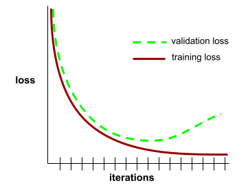
如需了解详情,请参阅机器学习速成课程中的泛化。
广义线性模型
一种基于其他类型噪声(例如 Poisson 噪声或类别噪声)的其他类型模型,是基于 Gaussian 噪声的最小二乘回归模型的泛化。广义线性模型的示例包括:
- 逻辑回归
- 多类别回归
- 最小二乘回归
可以通过凸优化找到广义线性模型的参数。
广义线性模型具有以下特性:
- 最优的最小二乘回归模型的平均预测结果等于训练数据的平均标签。
- 最优的逻辑回归模型预测的平均概率等于训练数据的平均标签。
广义线性模型的能力受其特征的限制。与深度模型不同,广义线性模型无法“学习新特征”。
生成的文本
一般来说,指机器学习模型输出的文本。在评估大型语言模型时,某些指标会将生成的文本与参考文本进行比较。例如,假设您要确定某个机器学习模型从法语翻译为荷兰语的有效性。在此示例中:
- 生成的文本是机器学习模型输出的荷兰语翻译。
- 参考文本是人工翻译人员(或软件)创建的荷兰语译文。
请注意,某些评估策略不涉及参考文本。
生成对抗网络 (GAN)
一种用于创建新数据的系统,其中生成器负责创建数据,而判别器负责确定创建的数据是否有效。
如需了解详情,请参阅生成对抗网络课程。
生成式智能体(拟像)
智能体具有独特的角色、记忆和日常安排,可模拟真实的人类行为。
如需了解详情,请参阅生成式代理:人类行为的交互式模拟。
生成式 AI
一个新兴的变革性领域,没有正式定义。 不过,大多数专家都认为,生成式 AI 模型可以创建(“生成”)以下类型的内容:
- 复杂
- 连贯
- 原图
生成式 AI 的示例包括:
- 大语言模型,可以生成复杂的原创文本并回答问题。
- 图片生成模型,可生成独一无二的图片。
- 音频和音乐生成模型,可以创作原创音乐或生成逼真的语音。
- 视频生成模型,可生成原创视频。
一些较早的技术(包括 LSTM 和 RNN)也可以生成原创且连贯的内容。一些专家认为这些早期技术属于生成式 AI,而另一些专家则认为,真正的生成式 AI 需要生成比这些早期技术更复杂的输出。
与预测性机器学习相对。
生成模型
实际上是指执行以下任一操作的模型:
- 从训练数据集创建(生成)新样本。 例如,用诗歌数据集进行训练后,生成模型可以创作诗歌。生成对抗网络的生成器部分属于此类别。
- 确定新样本来自训练集或通过创建训练集的机制创建的概率。例如,用包含英文句子的数据集进行训练后,生成模型可确定新输入是有效英文句子的概率。
从理论上讲,生成模型可以辨别数据集中样本或特定特征的分布情况。具体来说:
p(examples)
无监督学习模型属于生成模型。
与判别模型相对。
生成器
与判别模型相对。
Gini 不纯度
与 entropy 类似的指标。拆分器使用从 Gini 不纯度或熵派生的值来为分类决策树组成条件。 信息增益源自熵。对于从 Gini 不纯度派生的指标,目前还没有普遍接受的等效术语;不过,这个未命名的指标与信息增益同样重要。
Gini 不纯度也称为 Gini 指数,或简称为 Gini。
黄金数据集
一组人工整理的数据,用于捕获标准答案。团队可以使用一个或多个黄金数据集来评估模型的质量。
有些黄金数据集捕获了标准答案的不同子网域。例如,用于图片分类的黄金数据集可能会捕获光照条件和图片分辨率。
黄金回答
2 + 2
理想的回答是:
4
Google AI Studio
一款 Google 工具,提供简单易用的界面,可用于测试和构建使用 Google 大语言模型的应用。 如需了解详情,请参阅 Google AI Studio 首页。
GPT(生成式预训练转换器)
由 OpenAI 开发的一系列基于 Transformer 的大语言模型。
GPT 变体可应用于多种模态,包括:
- 图片生成(例如 ImageGPT)
- 文生图(例如 DALL-E)。
渐变色
相对于所有自变量的偏导数向量。在机器学习中,梯度是模型函数偏导数的向量。梯度指向最高速上升的方向。
梯度累积
一种反向传播技术,它仅在每个周期更新一次参数,而不是在每次迭代时更新。在处理每个 小批次 后,梯度累积只会更新梯度总和。然后,在处理完周期中的最后一个小批次后,系统最终会根据所有梯度变化的总和来更新参数。
当批次大小与可用于训练的内存量相比非常大时,梯度累积非常有用。当内存出现问题时,人们自然会倾向于减小批次大小。不过,在正常反向传播中,减小批次大小会增加参数更新次数。梯度累积使模型能够避免内存问题,同时仍能高效训练。
梯度提升(决策)树 (GBT)
一种决策森林,其中:
如需了解详情,请参阅决策森林课程中的梯度提升决策树。
梯度提升
一种训练算法,其中训练弱模型以迭代方式提高强模型的质量(减少损失)。例如,弱模型可以是线性模型或小型决策树模型。强模型成为之前训练的所有弱模型的总和。
在最简单的梯度提升形式中,每次迭代都会训练一个弱模型来预测强模型的损失梯度。然后,通过减去预测梯度来更新强模型的输出,类似于梯度下降法。
其中:
- $F_{0}$ 是初始强模型。
- $F_{i+1}$ 是下一个强模型。
- $F_{i}$ 是当前的强模型。
- $\xi$ 是一个介于 0.0 和 1.0 之间的值,称为收缩率,类似于梯度下降中的学习率。
- $f_{i}$ 是经过训练的弱模型,用于预测 $F_{i}$ 的损失梯度。
梯度提升的现代变体还在计算中纳入了损失的二阶导数(Hessian)。
决策树通常用作梯度提升中的弱模型。请参阅梯度提升(决策)树。
梯度裁剪
一种常用机制,用于在通过梯度下降法来训练模型时,通过人为限制(剪裁)梯度的最大值来缓解梯度爆炸问题。
梯度下降法
一种用于最大限度减少损失的数学技术。梯度下降法以迭代方式调整权重和偏差,逐渐找到可将损失降至最低的最佳组合。
梯度下降法比机器学习早得多。
如需了解详情,请参阅机器学习速成课程中的线性回归:梯度下降。
图表
TensorFlow 中的一种计算规范。图中的节点表示操作。边缘具有方向,表示将某项操作的结果(一个Tensor)作为一个操作数传递给另一项操作。可以使用 TensorBoard 可视化图。
图执行
一种 TensorFlow 编程环境,在该环境中,图执行程序会先构造一个图,然后执行该图的所有部分或某些部分。图执行是 TensorFlow 1.x 中的默认执行模式。
与即刻执行相对。
贪婪策略
标准答案关联性
一种模型的属性,其输出基于(“基于”)特定的素材。例如,假设您向大语言模型提供了一本完整的物理教科书作为输入(“上下文”)。然后,您向该大语言模型提出一个物理学问题。 如果模型的回答反映了该教科书中的信息,则表示该模型以该教科书为依据。
请注意,接地模型并不总是事实模型。例如,输入的物理教科书可能包含错误。
grounding
根据从一个或多个可信来源检索到的信息来生成 LLM 的全部或部分回答的过程。 例如,假设用户提示 LLM 提供柏林今天的天气预报。LLM 可能会根据从欧洲中期天气预报中心收集的信息来生成回答。
检索增强生成 (RAG) 是一种常用的接地技术。
标准答案
现实。
实际发生的事情。
例如,假设有一个二元分类模型,用于预测大学一年级学生是否会在六年内毕业。此模型的标准答案是相应学生是否在 6 年内实际毕业。
群体归因偏差
假设某个人的真实情况适用于相应群体中的每个人。如果使用便利抽样收集数据,群体归因偏差的影响会加剧。在非代表性样本中,归因可能不会反映现实。
另请参阅群外同质性偏差和群内偏差。另请参阅机器学习速成课程中的公平性:偏差类型,了解详情。
保护措施
可防止对人类或系统造成伤害的任何软件或流程。 危害可能有多种表现形式,包括防止数据泄露或未经授权的访问,或确保 LLM 的回答不包含令人反感的内容。
H
幻觉
生成式 AI 模型生成看似合理但实际上不正确的输出,并且声称对现实世界做出断言。例如,如果生成式 AI 模型声称巴拉克·奥巴马于 1865 年去世,则表示该模型出现了幻觉。
哈希技术
机器学习中对分类数据进行分桶的机制,尤其适合以下情形:类别数量庞大,但实际出现在数据集中的类别数量相对较小。
例如,地球上约有 7.3 万种树。您可以用 7.3 万个单独的分类桶表示所有 7.3 万种树中的每一种。或者,如果实际出现在数据集中的树只有 200 种,您可以进行哈希处理,将这些树种划分到约 500 个桶中。
一个桶可能包含多个树种。例如,哈希可能会将“猴面包树”和“红枫”这两个基因相异的树种放入同一个桶中。无论如何,哈希仍然是将大型分类集合映射到所选数量的桶的好方法。通过以确定的方式对值进行分组,哈希将具有大量可能值的分类特征变为更少数量的值。
如需了解详情,请参阅机器学习速成课程中的分类数据:词汇和独热编码。
启发法
一种简单且可快速实施的问题解决方案。例如,“采用启发法,我们实现了 86% 准确率。当我们改为使用深度神经网络时,准确率上升到 98%。”
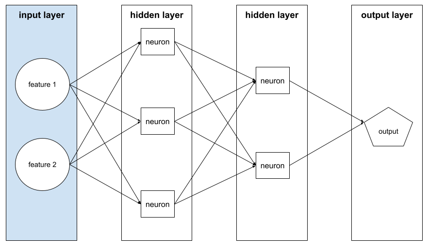
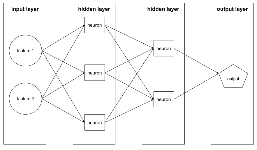
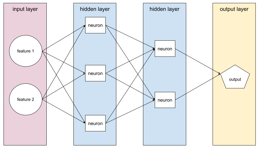
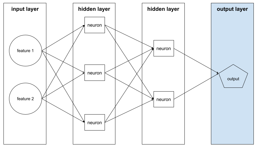
隐藏层
神经网络中介于输入层(特征)和输出层(预测)之间的层。每个隐藏层都包含一个或多个神经元。例如,以下神经网络包含两个隐藏层,第一个隐藏层有 3 个神经元,第二个隐藏层有 2 个神经元:
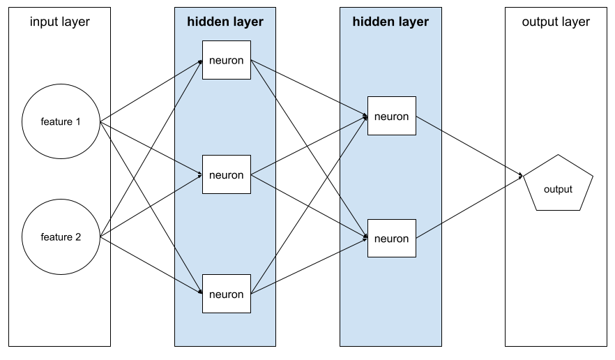
深度神经网络包含多个隐藏层。例如,上图所示的是一个深度神经网络,因为该模型包含两个隐藏层。
如需了解详情,请参阅机器学习速成课程中的神经网络:节点和隐藏层。
层次聚类
一类聚类算法,用于创建聚类树。层次聚类非常适合分层数据,例如植物分类。层次聚类算法有两种类型:
- 凝聚式层次聚类首先将每个样本分配到其自己的聚类,然后以迭代方式合并最近的聚类,以创建层次树。
- 分裂式层次聚类首先将所有样本分组到一个聚类,然后以迭代方式将该聚类划分为一个层次树。
与形心聚类相对。
如需了解详情,请参阅聚类课程中的聚类算法。
爬坡
一种用于以迭代方式改进(“爬山”)机器学习模型的算法,直到模型不再改进(“到达山顶”)为止。该算法的一般形式如下:
- 构建初始模型。
- 通过对训练或微调方式进行小幅调整,创建新的候选模型。这可能需要使用略有不同的训练集或不同的超参数。
- 评估新的候选模型,然后执行以下某项操作:
- 如果候选模型的表现优于初始模型,则该候选模型会成为新的初始模型。在这种情况下,请重复第 1 步、第 2 步和第 3 步。
- 如果没有模型优于初始模型,则说明您已到达山顶,应停止迭代。
如需有关超参数调节的指导,请参阅深度学习调优实战手册。如需有关特征工程的指导,请参阅机器学习速成课程的数据模块。
合页损失函数
一类用于分类的损失函数,旨在找到尽可能远离每个训练示例的决策边界,从而使示例和边界之间的边距最大化。核支持向量机使用合页损失函数(或相关函数,例如平方合页损失函数)。对于二元分类,合页损失函数的定义如下:
其中,y 是真实标签(-1 或 +1),y' 是分类模型的原始输出:
因此,合页损失函数与 (y * y') 的对比图如下所示:

历史偏差
一种已经存在于现实世界中并已进入数据集的偏见。这些偏差往往会反映出既有的文化刻板印象、人口统计学不平等以及对某些社会群体的偏见。
例如,假设有一个分类模型,用于预测贷款申请人是否会拖欠贷款,该模型是根据 20 世纪 80 年代来自两个不同社区的本地银行的历史贷款违约数据训练而成的。如果社区 A 的过往申请人拖欠贷款的可能性是社区 B 的申请人的 6 倍,模型可能会学习到历史偏差,导致模型不太可能批准社区 A 的贷款,即使导致该社区拖欠率较高的历史条件已不再相关。
如需了解详情,请参阅机器学习速成课程中的公平性:偏差类型。
留出数据
训练期间故意不使用(“留出”)的样本。验证数据集和测试数据集都属于留出数据。留出数据有助于评估模型向训练时所用数据之外的数据进行泛化的能力。与基于训练数据集的损失相比,基于留出数据集的损失有助于更好地估算基于未见过的数据集的损失。
主机
在加速器芯片(GPU 或 TPU)上训练机器学习模型时,系统中负责控制以下两方面的部分:
- 代码的总体流程。
- 输入流水线的提取和转换。
主机通常在 CPU 上运行,而不是在加速器芯片上运行;设备在加速器芯片上处理张量。
人工评估
一种由人来评判机器学习模型输出质量的过程;例如,让双语人士评判机器学习翻译模型的质量。对于没有唯一正确答案的模型,人工评估尤其有用。
人机协同 (HITL)
一种定义宽泛的表达方式,可能表示以下任一含义:
- 以批判性或怀疑性态度看待生成式 AI 输出的政策。
- 一种策略或系统,用于确保人们帮助塑造、评估和改进模型的行为。人机协同可使 AI 同时受益于机器智能和人类智能。例如,在 AI 生成代码后由软件工程师审核的系统就是一个人机协同系统。
超参数
在模型训练的连续运行期间,您或超参数调节服务(例如 Vizier)调整的变量。例如,学习速率就是一种超参数。您可以在一次训练会话之前将学习速率设置为 0.01。如果您认为 0.01 过高,或许可以在下一次训练会话中将学习率设置为 0.003。
如需了解详情,请参阅机器学习速成课程中的线性回归:超参数。
超平面
将空间划分为两个子空间的边界。例如,直线是二维空间中的超平面,平面是三维空间中的超平面。 在机器学习中,超平面通常是分隔高维空间的边界。核支持向量机利用超平面将正类别和负类别区分开来(通常是在极高维度空间中)。
I
i.i.d.
独立同分布的缩写。
图像识别
对图像中的物体、图案或概念进行分类的过程。 图像识别也称为图像分类。
不平衡的数据集
与类别不平衡的数据集的含义相同。
隐性偏差
根据一个人的心智模式和记忆自动建立关联或做出假设。隐性偏差会影响以下方面:
- 数据的收集和分类方式。
- 机器学习系统的设计和开发方式。
例如,在构建用于识别婚礼照片的分类模型时,工程师可能会将照片中的白色裙子用作一个特征。不过,白色裙子只在某些时代和某些文化中是一种婚礼习俗。
另请参阅确认偏差。
插补
值插补的简写形式。
公平性指标互不相容
某些公平性概念互不相容,无法同时满足。因此,没有一种通用的指标可用于量化公平性,并适用于所有机器学习问题。
虽然这可能令人沮丧,但公平性指标互不相容并不意味着公平性方面的努力是徒劳的。相反,它表明必须根据特定机器学习问题的具体情况来定义公平性,目的是防止出现特定于其应用场景的危害。
如需更详细地了解公平性指标的不兼容性,请参阅“公平性的(不)可能性”。
上下文学习
与少样本提示的含义相同。
独立同分布 (i.i.d)
从不发生变化且每次抽取的值不依赖于之前抽取的值的分布中抽取的数据。i.i.d. 是机器学习的理想情况 - 一种实用的数学结构,但在现实世界中几乎从未发现过。例如,某个网页的访问者在短时间内的分布可能为 i.i.d.,即分布在该短时间内没有变化,且一位用户的访问行为通常与另一位用户的访问行为无关。不过,如果您扩大时间范围,网页访问者的季节性差异可能会显现出来。
另请参阅非平稳性。
个体公平性
一种公平性指标,用于检查相似的个体是否被归为相似的类别。例如,Brobdingnagian Academy 可能希望通过确保成绩和标准化考试分数完全相同的两名学生获得入学的可能性相同,来满足个人公平性。
请注意,个体公平性完全取决于您如何定义“相似性”(在本例中为成绩和考试分数),如果相似性指标遗漏了重要信息(例如学生课程的严格程度),您可能会引入新的公平性问题。
如需详细了解个体公平性,请参阅“通过感知实现公平”。
推理
在传统机器学习中,通过将训练过的模型应用于无标签样本来做出预测的过程。 如需了解详情,请参阅“机器学习简介”课程中的监督式学习。
在大语言模型中,推理是指使用训练好的模型针对输入提示生成回答的过程。
推理在统计学中具有略有不同的含义。如需了解详情,请参阅 维基百科中有关统计学推断的文章。
推理路径
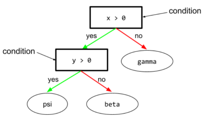
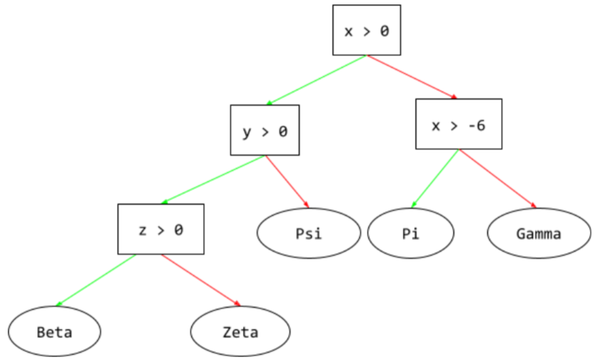
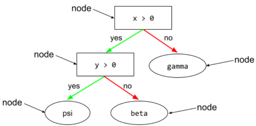
在决策树中,在推理过程中,特定示例从根到其他条件所采用的路线,最终以叶结束。例如,在以下决策树中,较粗的箭头显示了具有以下特征值的示例的推理路径:
- x = 7
- y = 12
- z = -3
下图中的推理路径在到达叶节点 (Zeta) 之前会经历三种情况。
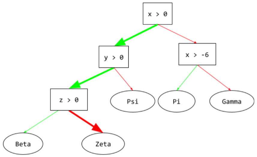
三条粗箭头显示了推理路径。
如需了解详情,请参阅“决策森林”课程中的决策树。
信息增益
在决策森林中,节点的熵与其子节点的熵(按示例数量加权)之和之间的差。节点的熵是指该节点中示例的熵。
例如,请考虑以下熵值:
- 父节点的熵 = 0.6
- 一个子节点的熵(有 16 个相关示例)= 0.2
- 另一个具有 24 个相关示例的子节点的熵 = 0.1
因此,40% 的示例位于一个子节点中,60% 的示例位于另一个子节点中。因此:
- 子节点的加权熵之和 = (0.4 * 0.2) + (0.6 * 0.1) = 0.14
因此,信息增益为:
- 信息增益 = 父节点的熵 - 子节点的加权熵之和
- 信息增益 = 0.6 - 0.14 = 0.46
群内偏差
对自身所属的群组或自身特征表现出偏向。 如果测试人员或评分者由机器学习开发者的好友、家人或同事组成,那么群内偏差可能会导致产品测试或数据集无效。
如需了解详情,请参阅机器学习速成课程中的公平性:偏差类型。
输入生成器
一种将数据加载到神经网络中的机制。
输入生成器可以看作是一个组件,负责将原始数据处理为张量,然后对这些张量进行迭代以生成用于训练、评估和推理的批次。
输入层
神经网络中用于存储特征向量的层。也就是说,输入层为训练或推理提供示例。例如,以下神经网络中的输入层包含两个特征:
在集合条件中
在决策树中,一种用于测试一组项中是否存在某个项的条件。例如,以下是一个集合内条件:
house-style in [tudor, colonial, cape]
在推理期间,如果房屋风格 特征的值为 tudor、colonial 或 cape,则此条件的评估结果为“是”。如果房屋风格特征的值为其他值(例如 ranch),则此条件的计算结果为“否”。
与测试独热编码特征的条件相比,集合内条件通常会生成更高效的决策树。
实例
与示例的含义相同。
指令调优
一种微调形式,可提高生成式 AI 模型遵循指令的能力。指令调优是指使用一系列指令提示训练模型,这些指令提示通常涵盖各种各样的任务。经过指令调优的模型往往能够针对各种任务的零样本提示生成实用的回答。
比较和对比:
可解释性
能够以人类可理解的方式解释或呈现机器学习模型的推理过程。
例如,大多数线性回归模型都具有很高的可解释性。(您只需查看每个特征的训练权重。)决策森林也具有很高的可解释性。不过,某些模型仍需进行复杂的可视化处理,才能变得可解释。
您可以使用 Learning Interpretability Tool (LIT) 来解读机器学习模型。
评分者间一致性信度
衡量人工标注者在执行任务时达成一致的频率。 如果评分者意见不一致,可能需要改进任务说明。 有时也称为注释者间一致性信度或评分者间可靠性信度。另请参阅 Cohen's kappa(最热门的评分者间一致性信度衡量指标之一)。
如需了解详情,请参阅机器学习速成课程中的分类数据:常见问题。
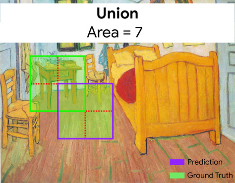
交并比 (IoU)
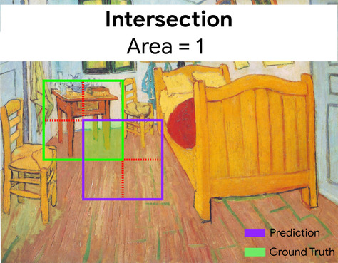
两个集合的交集除以并集。在机器学习图像检测任务中,IoU 用于衡量模型预测的边界框相对于标准答案边界框的准确率。在这种情况下,两个框的 IoU 是重叠面积与总面积的比值,其值范围为 0(预测的边界框与标准答案边界框不重叠)到 1(预测的边界框与标准答案边界框的坐标完全相同)。
例如,在下图中:
- 预测的边界框(用于界定模型预测的画作中床头柜所在位置的坐标)以紫色轮廓显示。
- 标准答案边界框(用于界定画作中床头柜实际所在位置的坐标)以绿色轮廓显示。
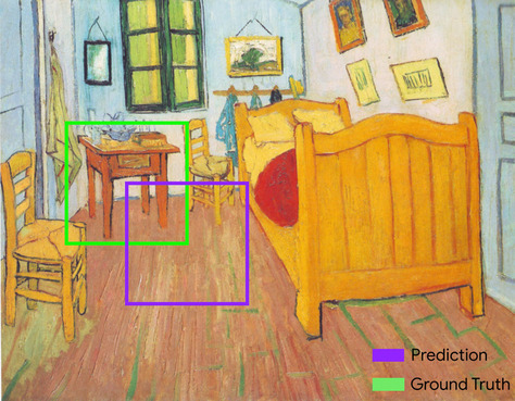
在此示例中,预测和标准答案的边界框的交集(左下图)为 1,预测和标准答案的边界框的并集(右下图)为 7,因此 IoU 为 \(\frac{1}{7}\)。
IoU
交并比的缩写。
商品矩阵
在推荐系统中,由矩阵分解生成的嵌入向量矩阵,其中包含有关每个推荐项的潜在信号。项矩阵的每一行都包含所有推荐项的单个潜在特征的值。以电影推荐系统为例。项矩阵中的每一列表示一部电影。潜在信号可能表示类型,也可能是更难以解读的信号,其中涉及类型、明星、影片年代或其他因素之间的复杂互动关系。
项矩阵与要进行分解的目标矩阵具有相同的列数。例如,假设某个影片推荐系统要评估 10000 部影片,则项矩阵会有 10000 个列。
项目
在推荐系统中,系统推荐的实体。例如,视频是音像店推荐的推荐项,而书籍是书店推荐的推荐项。
迭代
在训练期间,对模型的参数(即模型的权重和偏差)进行一次更新。批次大小决定了模型在单次迭代中处理的样本数量。例如,如果批次大小为 20,则模型会在调整参数之前处理 20 个样本。
在训练神经网络时,单次迭代涉及以下两个传递:
- 一次前向传递,用于评估单个批次的损失。
- 一次反向传递(反向传播),用于根据损失和学习速率调整模型参数。
如需了解详情,请参阅机器学习速成课程中的梯度下降。
J
JAX
一个数组计算库,将 XLA(加速线性代数)和自动微分功能结合在一起,实现高性能数值计算。JAX 提供了一个简单而强大的 API,用于编写具有可组合转换的加速数值代码。JAX 提供以下功能:
grad(自动微分)jit(即时编译)vmap(自动矢量化或批处理)pmap(并行化)
JAX 是一种用于表达和组合数值代码转换的语言,类似于 Python 的 NumPy 库,但范围要大得多。(事实上,JAX 下的 .numpy 库是 Python NumPy 库的功能等效但完全重写的版本。)
JAX 通过将模型和数据转换为适合在 GPU 和 TPU 加速器芯片上并行处理的形式,特别适合加速许多机器学习任务。
Flax、Optax、Pax 和许多其他库都基于 JAX 基础架构构建。
K
Keras
一种热门的 Python 机器学习 API。Keras 能够在多种深度学习框架上运行,其中包括 TensorFlow(在该框架上,Keras 作为 tf.keras 提供)。
核支持向量机 (KSVM)
一种分类算法,旨在通过将输入数据向量映射到更高维度的空间,最大限度地扩大正类别和负类别之间的边际。以某个输入数据集包含一百个特征的分类问题为例。为了最大化正类别和负类别之间的边际,核支持向量机可以在内部将这些特征映射到百万维度的空间。核支持向量机使用合页损失函数。
关键点
图片中特定特征的坐标。例如,对于区分花卉种类的图像识别模型,关键点可能是每个花瓣的中心、花茎、雄蕊等。
k 折叠交叉验证
一种用于预测模型泛化到新数据的能力的算法。k 折交叉验证中的 k 是指您将数据集的示例划分成的相等组数;也就是说,您将训练和测试模型 k 次。在每轮训练和测试中,一个不同的组是测试集,所有剩余的组都成为训练集。经过 k 轮训练和测试后,计算所选测试指标的平均值和标准差。
例如,假设您的数据集包含 120 个示例。进一步假设,您决定将 k 设置为 4。因此,在对示例进行随机排序后,您将数据集划分为四个包含 30 个示例的相等组,并进行四轮训练和测试:
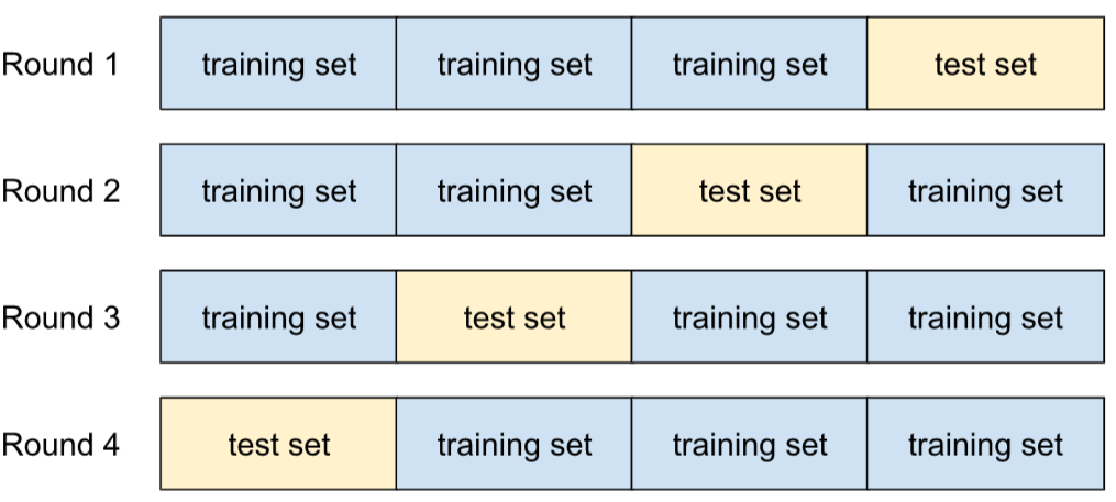
例如,均方误差 (MSE) 可能是线性回归模型中最有意义的指标。因此,您需要计算所有四轮的 MSE 的平均值和标准差。
k-means
一种热门的聚类算法,用于对无监督学习中的样本进行分组。k-means 算法基本上会执行以下操作:
- 以迭代方式确定最佳的 k 中心点(称为形心)。
- 将每个样本分配到最近的形心。与同一个形心距离最近的样本属于同一个组。
k-means 算法会挑选形心位置,以最大限度地减小每个样本与其最接近形心之间的距离的累积平方。
例如,请看以下狗身高与狗宽度的散点图:

如果 k=3,k-means 算法将确定三个形心。每个样本都会分配到离它最近的形心,从而产生三个组:

假设某制造商想要确定适合小型犬、中型犬和大型犬的毛衣的理想尺寸。这三个形心分别表示相应聚类中每只狗的平均身高和平均宽度。因此,制造商可能应根据这三个形心来确定毛衣尺码。请注意,聚类的形心通常不是聚类中的示例。
上图显示了仅包含两个特征(身高和体重)的示例的 k-means。请注意,K-means 可以跨多个特征对示例进行分组。
如需了解详情,请参阅聚类课程中的什么是 K-means 聚类?
k-median
与 k-means 紧密相关的聚类算法。两者的实际区别如下:
- 对于 k-means,确定形心的方法是,最大限度地减小候选形心与它的每个样本之间的距离平方和。
- 对于 k-median,确定形心的方法是,最大限度地减小候选形心与它的每个样本之间的距离总和。
请注意,距离的定义也有所不同:
- k-means 采用从形心到样本的欧几里得距离。(在二维空间中,欧几里得距离即使用勾股定理计算斜边。)例如,(2,2) 与 (5,-2) 之间的 k-means 距离为:
- k-median 采用从形心到样本的 曼哈顿距离。这个距离是每个维度中绝对差值的总和。例如,(2,2) 与 (5,-2) 之间的 k-median 距离为:
L
L0 正则化
一种正则化,用于惩罚模型中非零权重的总数。例如,具有 11 个非零权重的模型受到的惩罚会高于具有 10 个非零权重的类似模型。
L0 正则化有时称为 L0 范数正则化。
L1 损失
一种损失函数,用于计算实际标签值与模型预测的值之间的差的绝对值。例如,以下是针对包含 5 个示例的批次计算 L1 损失的示例:
| 示例的实际值 | 模型的预测值 | 增量的绝对值 |
|---|---|---|
| 7 | 6 | 1 |
| 5 | 4 | 1 |
| 8 | 11 | 3 |
| 4 | 6 | 2 |
| 9 | 8 | 1 |
| 8 = L1 损失 | ||
平均绝对误差是指每个样本的平均 L1 损失。
如需了解详情,请参阅机器学习速成课程中的线性回归:损失。
L1 正则化
一种正则化,根据权重的绝对值总和按比例惩罚权重。L1 正则化有助于使不相关或几乎不相关的特征的权重正好为 0。权重为 0 的特征实际上已从模型中移除。
与 L2 正则化相对。
L2 损失
一种损失函数,用于计算实际标签值与模型预测的值之间的平方差。例如,以下是针对包含 5 个示例的批次计算 L2 损失的示例:
| 示例的实际值 | 模型的预测值 | 增量的平方 |
|---|---|---|
| 7 | 6 | 1 |
| 5 | 4 | 1 |
| 8 | 11 | 9 |
| 4 | 6 | 4 |
| 9 | 8 | 1 |
| 16 = L2 损失 | ||
由于取平方值,因此 L2 损失会放大离群值的影响。也就是说,与 L1 损失相比,L2 损失对不良预测的反应更强烈。例如,前一个批次的 L1 损失将为 8 而不是 16。请注意,一个离群值就占了 16 个值中的 9 个。
回归模型通常使用 L2 损失作为损失函数。
均方误差是指每个样本的平均 L2 损失。 平方损失是 L2 损失的另一种称法。
如需了解详情,请参阅机器学习速成课程中的逻辑回归:损失和正则化。
L2 正则化
一种正则化,根据权重的平方和按比例惩罚权重。L2 正则化有助于使离群值(具有较大正值或较小负值)权重接近 0,但又不正好为 0。值非常接近 0 的特征会保留在模型中,但对模型的预测影响不大。
L2 正则化始终可以提高线性模型的泛化能力。
与 L1 正则化相对。
如需了解详情,请参阅机器学习速成课程中的过拟合:L2 正则化。
标签
每个有标签样本都包含一个或多个特征和一个标签。例如,在垃圾邮件检测数据集中,标签可能是“垃圾邮件”或“非垃圾邮件”。在降雨量数据集中,标签可能是特定时间段内的降雨量。
如需了解详情,请参阅《机器学习简介》中的监督式学习。
有标签样本
包含一个或多个特征和一个标签的示例。例如,下表显示了房屋估值模型中的三个带标签的示例,每个示例都包含三个特征和一个标签:
| 卧室数量 | 浴室数量 | 房屋年龄 | 房价(标签) |
|---|---|---|---|
| 3 | 2 | 15 | $345,000 |
| 2 | 1 | 72 | 17.9 万美元 |
| 4 | 2 | 34 | 39.2 万美元 |
在监督式机器学习中,模型基于带标签的样本进行训练,并基于无标签的样本进行预测。
将有标签样本与无标签样本进行对比。
如需了解详情,请参阅《机器学习简介》中的监督式学习。
标签泄露
一种模型设计缺陷,其中特征是标签的代理。例如,假设有一个二元分类模型,用于预测潜在客户是否会购买特定产品。假设模型的某个特征是一个名为 SpokeToCustomerAgent 的布尔值。进一步假设,只有在潜在客户实际购买产品后,才会为其分配客户服务人员。在训练期间,模型将快速学习 SpokeToCustomerAgent 与标签之间的关联。
如需了解详情,请参阅机器学习速成课程中的监控流水线。
lambda
与正则化率的含义相同。
Lambda 是一个过载的术语。我们在此关注的是该术语在正则化中的定义。
LaMDA(对话应用语言模型)
由 Google 开发的基于 Transformer 的大语言模型,经过大型对话数据集训练,可生成逼真的对话回答。
LaMDA:我们富有突破性的对话技术提供了概览。
landmarks
与关键点的含义相同。
语言模型
一种用于估计较长的 token 序列中出现某个 token 或 token 序列的概率的模型。
如需了解详情,请参阅机器学习速成课程中的什么是语言模型?。
大语言模型
至少是一个具有大量参数的语言模型。更通俗地说,任何基于 Transformer 的语言模型,例如 Gemini 或 GPT。
如需了解详情,请参阅机器学习速成课程中的大语言模型 (LLM)。
延迟时间
模型处理输入并生成回答所需的时间。 高延迟响应的生成时间比低延迟响应长。
影响大语言模型延迟时间的因素包括:
- 输入和输出 token 长度
- 模型的复杂程度
- 模型运行的基础设施
优化延迟时间对于打造响应迅速且人性化的应用至关重要。
潜在空间
与嵌入空间的含义相同。
图层
例如,下图展示了一个包含 1 个输入层、2 个隐藏层和 1 个输出层的神经网络:
在 TensorFlow 中,层也是 Python 函数,以张量和配置选项作为输入,然后生成其他张量作为输出。
Layers API (tf.layers)
一种 TensorFlow API,用于以层组合的方式构建深度神经网络。通过 Layers API,您可以构建不同类型的层,例如:
tf.layers.Dense用于全连接层。tf.layers.Conv2D(适用于卷积层)。
Layers API 遵循 Keras Layers API 规范。 也就是说,除了前缀不同之外,Layers API 中的所有函数都具有与 Keras layers API 中对应的函数相同的名称和签名。
leaf
决策树中的任何端点。与条件不同,叶不执行测试。相反,叶节点是一种可能的预测。叶也是推理路径的终端节点。
例如,以下决策树包含三个叶节点:
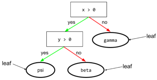
如需了解详情,请参阅“决策森林”课程中的决策树。
Learning Interpretability Tool (LIT)
一种直观的交互式模型理解和数据可视化工具。
您可以使用开源 LIT 来解读模型,或直观呈现文本、图片和表格数据。
学习速率
一个浮点数,用于告知梯度下降法算法在每次迭代时调整权重和偏差的幅度。例如,0.3 的学习速率调整权重和偏差的力度是 0.1 的学习速率的三倍。
学习速率是一个重要的超参数。如果您将学习速率设置得过低,训练将耗时过长。如果您将学习速率设置得过高,梯度下降法通常难以实现收敛。
如需了解详情,请参阅机器学习速成课程中的线性回归:超参数。
最小二乘回归
由简入繁的提示
一种提示链形式,可将复杂问题分解为一组有序的简单问题。例如,以下是针对特定问题的从最少到最多的提示策略:
- 将复杂问题分解为一系列按顺序排列的较简单子问题。 在此示例中,假设有 3 个子问题。
- 提示 1:让 LLM 解决第一个子问题。LLM 返回回答 1。
- 提示 2:将回答 1 的全部或部分内容整合到提示中,以解决第二个子问题。LLM 返回回答 2。
- 提示 3:将回答 2 的全部或部分内容整合到提示中,以解决第三个子问题。LLM 对提示 3 的回答是初始复杂问题的“最终”答案。
请注意,每个步骤都依赖于上一步的解决方案。
与思维链提示相对。
Levenshtein 距离
一种编辑距离指标,用于计算将一个字词更改为另一个字词所需的最少删除、插入和替换操作次数。例如,“heart”和“darts”这两个字之间的 Levenshtein 距离为 3,因为以下 3 次编辑是将一个字转换为另一个字所需的最少更改次数:
- heart → deart(将“h”替换为“d”)
- deart → dart(删除“e”)
- dart → darts(插入“s”)
请注意,上述序列并非唯一包含 3 次编辑的路径。
线性
一种仅通过加法和乘法即可表示的两个或多个变量之间的关系。
线性关系的图是一条直线。
与非线性相对。
线性模型
一种为每个特征分配一个权重以进行预测的模型。(线性模型还包含偏差。)相比之下,深度模型中特征与预测的关系通常是非线性的。
线性模型通常比深度模型更易于训练,并且可解释性更强。不过,深度模型可以学习特征之间的复杂关系。
线性回归
一种机器学习模型,同时满足以下两个条件:
将线性回归与逻辑回归进行对比。 此外,还要将回归与分类进行对比。
如需了解详情,请参阅机器学习速成课程中的线性回归。
LIT
Learning Interpretability Tool (LIT) 的缩写,之前称为 Language Interpretability Tool。
LLM
大语言模型的缩写。
LLM 评估
用于评估大型语言模型 (LLM) 性能的一组指标和基准。概括来讲,大语言模型评估:
- 帮助研究人员确定 LLM 需要改进的方面。
- 有助于比较不同的 LLM,并确定最适合特定任务的 LLM。
- 帮助确保 LLM 的使用安全且合乎道德。
如需了解详情,请参阅机器学习速成课程中的大型语言模型 (LLM)。
逻辑回归
一种可预测概率的回归模型。 逻辑回归模型具有以下特征:
- 标签为分类。逻辑回归一词通常是指二元逻辑回归,即计算具有两个可能值的标签的概率的模型。一种不太常见的变体是多项式逻辑回归,它用于计算具有两个以上可能值的标签的概率。
- 训练期间的损失函数为对数损失函数。(对于具有两个以上可能值的标签,可以并行放置多个对数损失函数单位。)
- 该模型采用线性架构,而非深度神经网络。不过,此定义的其余部分也适用于预测类别标签概率的深度模型。
例如,假设有一个逻辑回归模型,用于计算输入电子邮件是垃圾邮件或非垃圾邮件的概率。 在推理过程中,假设模型预测值为 0.72。因此,模型会估计:
- 电子邮件是垃圾邮件的概率为 72%。
- 电子邮件不是垃圾邮件的概率为 28%。
逻辑回归模型采用以下两步架构:
- 模型通过应用输入特征的线性函数来生成原始预测结果 (y')。
- 该模型使用原始预测作为 S 型函数的输入,该函数会将原始预测转换为介于 0 和 1 之间的值(不含 0 和 1)。
与任何回归模型一样,逻辑回归模型也会预测一个数值。不过,此数字通常会成为二元分类模型的一部分,如下所示:
- 如果预测的数值大于分类阈值,则二元分类模型会预测为正类别。
- 如果预测的数字小于分类阈值,二元分类模型会预测负类别。
如需了解详情,请参阅机器学习速成课程中的逻辑回归。
logits
分类模型生成的原始(未归一化)预测向量,通常随后会传递给归一化函数。如果模型要解决的是多类别分类问题,那么 logits 通常会成为 softmax 函数的输入。 然后,softmax 函数会生成一个(归一化)概率向量,其中每个可能类别对应一个值。
对数损失函数
如需了解详情,请参阅机器学习速成课程中的逻辑回归:损失和正则化。
对数几率
某个事件的对数几率。
长短期记忆 (LSTM)
循环神经网络中的一种细胞,用于在手写识别、机器翻译和图片说明等应用中处理数据序列。LSTM 通过在内部记忆状态中基于新输入和 RNN 中之前单元的上下文来维护历史记录,从而解决训练 RNN 时因数据序列过长而出现的梯度消失问题。
LoRA
低秩适应性的缩写。
损失
损失函数用于计算损失。
如需了解详情,请参阅机器学习速成课程中的线性回归:损失。
损失汇总器
一种机器学习算法,通过合并多个模型的预测结果并使用这些预测结果进行单个预测,来提高模型的性能。因此,损失聚合器可以减少预测的方差,并提高预测的准确率。
损失曲线
以训练迭代次数为自变量的损失函数图。下图显示了典型的损失曲线:
损失曲线可以绘制以下所有类型的损失:
另请参阅泛化曲线。
如需了解详情,请参阅机器学习速成课程中的过拟合:解读损失曲线。
损失函数
在训练或测试期间,用于计算一批示例的损失的数学函数。对于做出良好预测的模型,损失函数会返回较低的损失;对于做出不良预测的模型,损失函数会返回较高的损失。
训练的目标通常是尽量减少损失函数返回的损失。
损失函数有很多不同的种类。根据您要构建的模型类型选择合适的损失函数。例如:
损失曲面
权重与损失的图表。梯度下降法旨在找到损失曲面在局部最低点时的权重。
中间位置效应
LLM 更有效地使用长上下文窗口开头和结尾的信息,而不是中间的信息。也就是说,在给定长上下文的情况下,中间丢失效应会导致准确率:
- 当形成回答的相关信息位于上下文的开头或结尾附近时,相对较高。
- 当形成回答的相关信息位于上下文的中间时,为相对较低。
该术语源自《Lost in the Middle: How Language Models Use Long Contexts》(迷失在中间:语言模型如何使用长上下文)。
低秩自适应 (LoRA)
一种参数高效的微调技术,用于“冻结”模型的预训练权重(使其无法再被修改),然后在模型中插入一小部分可训练的权重。这组可训练的权重(也称为“更新矩阵”)比基础模型小得多,因此训练速度也快得多。
LoRA 具有以下优势:
- 提高模型在应用微调的网域中的预测质量。
- 与需要微调模型所有参数的技术相比,微调速度更快。
- 通过支持同时部署多个共享同一基础模型的专用模型,降低推理的计算成本。
LSTM
长短期记忆的缩写。
M
机器学习
一种通过输入数据训练模型的程序或系统。经过训练的模型可以根据从与训练该模型时使用的数据集具有相同分布的新(从未见过)数据集中提取的数据做出有用的预测。
机器学习还指与这些程序或系统相关的研究领域。
如需了解详情,请参阅机器学习简介课程。
机器翻译
使用软件(通常是机器学习模型)将文本从一种人类语言转换为另一种人类语言,例如从英语转换为日语。
多数类
类别不平衡的数据集内更为常见的标签。例如,假设一个数据集内包含 99% 的负标签和 1% 的正标签,那么负标签为多数类。
与少数类相对。
如需了解详情,请参阅机器学习速成课程中的数据集:不平衡的数据集。
经理代理
控制一个或多个子智能体的智能体。
马尔可夫决策过程 (MDP)
一种表示决策模型的图,其中做出决策(或采取行动)以在假设马尔可夫性质成立的情况下,浏览一系列状态。在强化学习中,这些状态之间的转换会返回数值奖励。
马尔可夫性质
某些环境的属性,其中状态转换完全由当前状态和智能体的动作中隐含的信息决定。
掩码语言模型
一种语言模型,用于预测候选令牌填入序列中空白处的概率。例如,遮盖语言模型可以计算候选字词的概率,以替换以下句子中的下划线:
帽子里的____回来了。
文献通常使用字符串“MASK”而不是下划线。 例如:
帽子上的“MASK”又回来了。
大多数现代掩码语言模型都是双向的。
math-pass@k
一种用于确定 LLM 在 K 次尝试内解决数学问题的准确性的指标。例如,math-pass@2 衡量的是 LLM 在两次尝试内解决数学问题的能力。在 math-pass@2 上达到 0.85 的准确率表明,LLM 在两次尝试中能够解决 85% 的数学问题。
math-pass@k 与 pass@k 指标相同,只不过 math-pass@k 专门用于数学评估。
matplotlib
一个开源 Python 2D 绘制库。matplotlib 可以帮助您可视化机器学习的各个不同方面。
矩阵分解
在数学中,矩阵分解是一种寻找其点积近似目标矩阵的矩阵的机制。
在推荐系统中,目标矩阵通常包含用户对商品的评分。例如,电影推荐系统的目标矩阵可能如下所示,其中正整数表示用户评分,0 表示用户未对该电影进行评分:
| 卡萨布兰卡 | 《旧欢新宠:费城故事》 | Black Panther | 神奇女侠 | 《低俗小说》 | |
|---|---|---|---|---|---|
| 用户 1 | 5.0 | 3.0 | 0.0 | 2.0 | 0.0 |
| 用户 2 | 4.0 | 0.0 | 0.0 | 1.0 | 5.0 |
| 用户 3 | 3.0 | 1.0 | 4.0 | 5.0 | 0.0 |
电影推荐系统旨在预测无评分电影的用户评分。例如,用户 1 会喜欢《黑豹》吗?
推荐系统采用的一种方法是,使用矩阵分解生成以下两个矩阵:
例如,对我们的三名用户和五个推荐项进行矩阵分解,会得到以下用户矩阵和项矩阵:
User Matrix                 Item Matrix

1.1   2.3           0.9   0.2   1.4    2.0   1.2
0.6   2.0           1.7   1.2   1.2   -0.1   2.1
2.5   0.5
用户矩阵和项矩阵的点积会得到一个推荐矩阵,其中不仅包含原始用户评分,还包含对每位用户未观看影片的预测。 例如,假设用户 1 对《卡萨布兰卡》的评分为 5.0。对应于推荐矩阵中该单元格的点积应该在 5.0 左右,计算方式如下:
(1.1 * 0.9) + (2.3 * 1.7) = 4.9更重要的是,用户 1 会喜欢《黑豹》吗?计算第一行和第三列所对应的点积,得到的预测评分为 4.3:
(1.1 * 1.4) + (2.3 * 1.2) = 4.3矩阵分解通常会生成用户矩阵和项矩阵,这两个矩阵合在一起明显比目标矩阵更为紧凑。
MBPP
Mostly Basic Python Problems 的缩写。
平均绝对误差 (MAE)
使用 L1 损失时,每个样本的平均损失。按如下方式计算平均绝对误差:
- 计算批次的 L1 损失。
- 将 L1 损失除以批次中的样本数。
例如,假设有以下一批包含 5 个示例的数据,请考虑计算 L1 损失:
| 示例的实际值 | 模型的预测值 | 损失(实际值与预测值之间的差值) |
|---|---|---|
| 7 | 6 | 1 |
| 5 | 4 | 1 |
| 8 | 11 | 3 |
| 4 | 6 | 2 |
| 9 | 8 | 1 |
| 8 = L1 损失 | ||
因此,L1 损失为 8,示例数量为 5。因此,平均绝对误差为:
Mean Absolute Error = L1 loss / Number of Examples
Mean Absolute Error = 8/5 = 1.6
前 k 名的平均精确率均值 (mAP@k)
验证数据集中所有 k 处的平均精确率得分的统计平均值。平均精确率(前 k 个)的一个用途是判断推荐系统生成的推荐的质量。
虽然“平均平均值”一词听起来有些冗余,但该指标的名称是合适的。毕竟,此指标会计算多个 k 值处的平均精确率的平均值。
均方误差 (MSE)
使用 L2 损失时,每个样本的平均损失。按如下方式计算均方误差:
- 计算批次的 L2 损失。
- 将 L2 损失除以批次中的样本数。
例如,假设以下一批包含 5 个示例,损失如下:
| 实际值 | 模型预测 | 损失 | 平方损失 |
|---|---|---|---|
| 7 | 6 | 1 | 1 |
| 5 | 4 | 1 | 1 |
| 8 | 11 | 3 | 9 |
| 4 | 6 | 2 | 4 |
| 9 | 8 | 1 | 1 |
| 16 = L2 损失 | |||
因此,均方误差为:
Mean Squared Error = L2 loss / Number of Examples
Mean Squared Error = 16/5 = 3.2
TensorFlow Playground 使用均方误差来计算损失值。
网格
在机器学习并行编程中,一个与将数据和模型分配给 TPU 芯片以及定义这些值将如何分片或复制相关的术语。
网格是一个多含义术语,可以理解为下列两种含义之一:
- TPU 芯片的物理布局。
- 一种用于将数据和模型映射到 TPU 芯片的抽象逻辑构造。
无论哪种情况,网格都被指定为形状。
元学习
一种发现或改进学习算法的机器学习子集。 元学习系统还可以旨在训练模型,使其能够从少量数据或从之前任务中获得的经验中快速学习新任务。元学习算法通常会尝试实现以下目标:
- 改进或学习人工设计的特征(例如初始化程序或优化器)。
- 提高数据效率和计算效率。
- 改善泛化效果。
元学习与少量样本学习有关。
指标
您关心的一项统计数据。
目标是机器学习系统尝试优化的指标。
Metrics API (tf.metrics)
用于评估模型的 TensorFlow API。例如,tf.metrics.accuracy 用于确定模型的预测与标签的匹配频率。
小批次
在一次迭代中处理的批次的一小部分随机选择的子集。 小批次的批次大小通常介于 10 到 1,000 个样本之间。
例如,假设整个训练集(完整批次)包含 1,000 个样本。进一步假设您将每个小批次的批次大小设置为 20。因此,每次迭代都会确定 1,000 个示例中随机 20 个示例的损失,然后相应地调整权重和偏差。
计算小批次的损失比计算完整批次中所有示例的损失要高效得多。
如需了解详情,请参阅机器学习速成课程中的线性回归:超参数。
小批次随机梯度下降法
一种使用小批次的梯度下降法。也就是说,小批次随机梯度下降法会根据一小部分训练数据估算梯度。常规随机梯度下降法使用的小批次的大小为 1。
minimax 损失
一种基于生成数据与真实数据分布之间的交叉熵的生成对抗网络的损失函数。
第一篇论文中使用了 minimax 损失来描述生成对抗网络。
如需了解详情,请参阅生成对抗网络课程中的损失函数。
少数类
类别不平衡的数据集中不常见的标签。例如,假设一个数据集内包含 99% 的负标签和 1% 的正标签,那么正标签为少数类。
与多数类相对。
如需了解详情,请参阅机器学习速成课程中的数据集:不平衡的数据集。
混合专家
一种通过仅使用一部分参数(称为“专家”)来处理给定输入令牌或示例来提高神经网络效率的方案。门控网络会将每个输入 token 或示例路由到合适的专家。
如需了解详情,请参阅以下任一论文:
机器学习
机器学习的缩写。
MMIT
多模态指令调优的缩写。
MNIST
由 LeCun、Cortes 和 Burges 编译的公用数据集,其中包含 60,000 张图像,每张图像显示人类如何手动写下从 0 到 9 的特定数字。每张图像存储为 28x28 的整数数组,其中每个整数是 0 到 255(含边界值)之间的灰度值。
MNIST 是机器学习的标准数据集,通常用于测试新的机器学习方法。如需了解详情,请参阅 MNIST 手写数字数据库。
modality
高级别数据类别。例如,数字、文字、图片、视频和音频是五种不同的模态。
模型
一般来说,任何处理输入数据并返回输出的数学结构。换句话说,模型是系统进行预测所需的一组形参和结构。 在监督式机器学习中,模型将示例作为输入,并推断出预测结果作为输出。在监督式机器学习中,模型略有不同。例如:
您可以保存、恢复或复制模型。
非监督式机器学习也会生成模型,通常是一个可以将输入示例映射到最合适的聚类的函数。
模型能力
模型可以学习的问题的复杂性。模型可以学习的问题越复杂,模型的能力就越高。模型能力通常会随着模型参数数量的增加而增强。如需了解分类模型容量的正式定义,请参阅 VC 维度。
模型级联
一种可为特定推理查询选择理想 模型的系统。
假设有一组模型,从非常大(大量形参)到小得多(形参少得多)。与较小的模型相比,超大型模型在推理时会消耗更多计算资源。不过,超大型模型通常可以推理出比小型模型更复杂的请求。模型级联会确定推理查询的复杂程度,然后选择合适的模型来执行推理。 模型级联的主要目的是通过选择较小的模型来降低推理费用,只有在处理更复杂的查询时才选择较大的模型。
假设有一个小型模型在手机上运行,而该模型的较大版本在远程服务器上运行。良好的模型级联可让较小的模型处理简单请求,仅在处理复杂请求时调用远程模型,从而降低成本和延迟时间。
另请参阅模型路由器。
模型并行处理
一种扩展训练或推理的方式,将一个模型的不同部分放在不同的设备上。模型并行化可实现无法在单个设备上运行的大型模型。
为了实现模型并行性,系统通常会执行以下操作:
- 将模型分片(划分)为更小的部分。
- 将这些较小部分的训练分配到多个处理器中。 每个处理器都会训练模型的一部分。
- 合并结果以创建单个模型。
模型并行处理会减慢训练速度。
另请参阅数据并行。
模型路由器
用于在模型级联中确定理想模型以进行推理的算法。 模型路由器本身通常是一个机器学习模型,它会逐渐学习如何为给定的输入选择最佳模型。不过,模型路由器有时可能是一种更简单的非机器学习算法。
模型训练
确定最佳模型的过程。
MOE
专家混合的缩写。
造势
一种复杂的梯度下降法,其中学习步长不仅取决于当前步长的导数,还取决于紧邻的前一步长(或多个步长)的导数。动量涉及计算梯度随时间的指数加权移动平均值,类似于物理学中的动量。动量有时可以防止学习陷入局部最小值。
Mostly Basic Python Problems (MBPP)
用于评估 LLM 在生成 Python 代码方面的熟练程度的数据集。 Mostly Basic Python Problems 提供了大约 1,000 个众包编程问题。 数据集中的每个问题都包含:
- 任务说明
- 解决方案代码
- 三个自动化测试用例
MT
机器翻译的缩写。
多智能体协作
一种框架,其中多个专业 AI 智能体相互互动、辩论或传递任务,以解决复杂问题。
多类别分类
在监督学习中,一种分类问题,其中数据集包含两个以上的标签类别。例如,Iris 数据集中的标签必须是以下三个类别之一:
- setosa 鸢尾花
- 弗吉尼亚鸢尾
- 杂色鸢尾
如果模型是使用 Iris 数据集训练的,并且可以根据新示例预测 Iris 类型,则该模型执行的是多类别分类。
相比之下,如果分类问题要区分的类别正好是两个,则属于二元分类模型。例如,预测电子邮件是垃圾邮件还是非垃圾邮件的电子邮件模型就是二元分类模型。
在聚类问题中,多类别分类是指两个以上的聚类。
如需了解详情,请参阅机器学习速成课程中的神经网络:多类别分类。
多类别逻辑回归
多头自注意力
自注意力的一种扩展,可针对输入序列中的每个位置多次应用自注意力机制。
Transformer 引入了多头自注意力机制。
多模态指令调优
一种经过指令调优的模型,可以处理文本以外的输入,例如图片、视频和音频。
多模态模型
输入、输出或两者都包含多种模态的模型。例如,假设有一个模型将图片和文本说明(两种模态)作为特征,并输出一个分数,用于指示文本说明与图片的匹配程度。因此,此模型的输入是多模态的,而输出是单模态的。
多项分类
与多类别分类的含义相同。
多项回归
与多类别逻辑回归的含义相同。
多句阅读理解 (MultiRC)
用于评估 LLM 回答多项选择题能力的数据集。 数据集中的每个示例都包含:
- 上下文段落
- 关于该段落的问题
- 问题的多个答案。每个答案都标有“正确”或“错误”。 多个答案可能为 True。
例如:
上下文段落:
苏珊想举办一个生日派对。她给所有朋友都打了电话。她有 5 个朋友。苏珊的妈妈说,苏珊可以邀请他们所有人参加派对。她的第一个朋友因生病而无法参加派对。她的第二个朋友要出差。她的第三个朋友不太确定父母是否会同意。第四位朋友回复了“不确定”。第五位朋友肯定会去参加聚会。苏珊有点难过。派对当天,这五位朋友都来了。每个朋友都给苏珊带了礼物。苏珊很高兴,并在下周给每位朋友寄了一张感谢卡。
问题:苏珊生病的朋友康复了吗?
多个答案:
- 是的,她已康复。(正确)
- 否。(False)
- 可以。(正确)
- 没有,她没有康复。(错误)
- 是的,她参加了苏珊的派对。(正确)
MultiRC 是 SuperGLUE 集成模型的一个组成部分。
如需了解详情,请参阅Looking Beyond the Surface: A Challenge Set for Reading Comprehension over Multiple Sentences。
多任务处理
多任务模型是通过训练适合每项不同任务的数据来创建的。这样一来,模型便可学习在不同任务之间共享信息,从而更有效地学习。
针对多项任务训练的模型通常具有更强的泛化能力,并且在处理不同类型的数据时更加稳健。
否
Nano
一款相对较小的 Gemini 模型,专为在设备上使用而设计。如需了解详情,请参阅 Gemini Nano。
NaN 陷阱
模型中的一个数字在训练期间变成 NaN,这会导致模型中的很多或所有其他数字最终也会变成 NaN。
NaN 是 Not a Number 的缩写。
自然语言处理
一个领域,旨在教导计算机使用语言规则来处理用户说出或输入的内容。几乎所有现代自然语言处理都依赖于机器学习。自然语言理解
自然语言处理的一个子集,用于确定所说或所输入内容的意图。自然语言理解可以超越自然语言处理,考虑语言的复杂方面,例如上下文、讽刺和情感。
负类别
在二元分类中,一种类别称为正类别,另一种类别称为负类别。正类别是模型正在测试的事物或事件,负类别则是另一种可能性。例如:
- 在医学检查中,负类别可以是“非肿瘤”。
- 在电子邮件分类模型中,负类别可以是“非垃圾邮件”。
与正类别相对。
负采样
与候选采样的含义相同。
神经架构搜索 (NAS)
一种用于自动设计神经网络架构的技术。NAS 算法可以减少训练神经网络所需的时间和资源。
NAS 通常使用:
- 搜索空间,即一组可能的架构。
- 一种适应度函数,用于衡量特定架构在给定任务上的表现。
NAS 算法通常从一小部分可能的架构开始,随着算法对有效架构的了解不断深入,逐渐扩大搜索空间。适应度函数通常基于架构在训练集上的性能,而算法通常使用强化学习技术进行训练。
事实证明,NAS 算法能够有效地为各种任务(包括图像分类、文本分类和机器翻译)找到高性能的架构。
输出表示
包含至少一个隐藏层的模型。深度神经网络是一种包含多个隐藏层的神经网络。例如,下图显示了一个包含两个隐藏层的深度神经网络。
神经网络中的每个神经元都会连接到下一层中的所有节点。例如,在上图中,请注意第一个隐藏层中的每个神经元都分别连接到第二个隐藏层中的两个神经元。
在计算机上实现的神经网络有时称为人工神经网络,以区别于大脑和其他神经系统中的神经网络。
某些神经网络可以模拟不同特征与标签之间极其复杂的非线性关系。
如需了解详情,请参阅机器学习速成课程中的神经网络。
神经元
在机器学习中,指神经网络的隐藏层中的一个独立单元。每个神经元都会执行以下两步操作:
第一个隐藏层中的神经元接受来自输入层中特征值的输入。任何隐藏层(第一个隐藏层除外)中的神经元都会接受前一个隐藏层中神经元的输入。例如,第二个隐藏层中的神经元接受来自第一个隐藏层中神经元的输入。
下图突出显示了两个神经元及其输入。
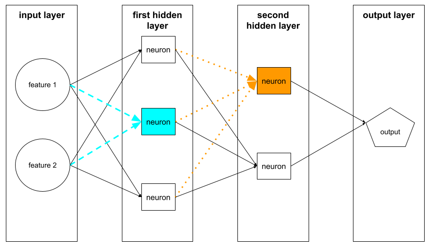
神经网络中的神经元会模拟大脑和神经系统其他部位的神经元的行为。
N-gram
N 个字词的有序序列。例如,“truly madly”属于二元语法。由于顺序很重要,因此“madly truly”和“truly madly”是不同的二元语法。
| 否 | 此类 N 元语法的名称 | 示例 |
|---|---|---|
| 2 | 二元语法 | to go、go to、eat lunch、eat dinner |
| 3 | 三元语法 | ate too much、happily ever after、the bell tolls |
| 4 | 四元语法 | walk in the park、dust in the wind、the boy ate lentils |
很多自然语言理解模型依赖 N 元语法来预测用户将输入或说出的下一个字词。例如,假设用户输入了“happily ever”。 基于三元语法的 NLU 模型可能会预测该用户接下来将输入“after”一词。
N 元语法与词袋(无序字词集)相对。
如需了解详情,请参阅机器学习速成课程中的大型语言模型。
NLP
自然语言处理的缩写。
NLU
自然语言理解的缩写。
节点(决策树)
如需了解详情,请参阅决策森林课程中的决策树。
节点(神经网络)
如需了解详情,请参阅机器学习速成课程中的神经网络。
节点(TensorFlow 图)
TensorFlow 图中的操作。
噪声
一般来说,噪声是指数据集中掩盖信号的所有内容。将噪声引入数据中的方式各种各样。例如:
- 人工评分者在添加标签时出错。
- 人类和仪器错误记录或忽略特征值。
非二元性别条件
包含两种以上可能结果的 条件。例如,以下非二元条件包含三种可能的结果:
如需了解详情,请参阅决策森林课程中的条件类型。
非确定性的
无法保证针对给定输入返回相同输出的系统。LLM 通常是非确定性的;也就是说,LLM 通常会针对同一提示生成不同的回答。
与确定性系统相比,不确定性系统通常更难测试。
另请参阅概率性。
非线性
一种无法仅通过加法和乘法表示的两个或多个变量之间的关系。线性关系可以用直线表示,而非线性关系则不能用直线表示。例如,假设有两个模型,每个模型都将单个特征与单个标签相关联。左侧的模型是线性模型,右侧的模型是非线性模型:

如需尝试不同类型的非线性函数,请参阅机器学习速成课程中的神经网络:节点和隐藏层。
无反应误差
请参阅选择性偏差。
非平稳性
一种值会随一个或多个维度(通常是时间)而变化的特征。 例如,请考虑以下非平稳性示例:
- 特定商店的泳衣销量会随季节而变化。
- 特定地区中特定水果的收获量在一年中的大部分时间为零,但在短时间内会很大。
- 由于气候变化,年平均气温正在发生变化。
与平稳性相对。
没有唯一正确答案 (NORA)
具有多个正确回答的提示。 例如,以下提示没有唯一正确的答案:
给我讲个关于大象的有趣笑话。
评估“没有唯一正确答案”问题的回答通常比评估有唯一正确答案的问题的回答更具主观性。例如,评估一个大象笑话需要一种系统性的方法来确定该笑话有多好笑。
NORA
没有唯一正确答案的缩写。
归一化
从广义上讲,是将变量的实际值范围转换为标准值范围的过程,例如:
- -1 至 +1
- 0 至 1
- Z 得分(大致介于 -3 到 +3 之间)
例如,假设某个特征的实际值范围为 800 到 2,400。作为特征工程的一部分,您可以将实际值归一化到标准范围内,例如 -1 到 +1。
归一化是特征工程中的一项常见任务。如果特征向量中的每个数值特征都具有大致相同的范围,模型通常会更快地完成训练(并生成更好的预测结果)。
另请参阅 Z 得分归一化。
如需了解详情,请参阅机器学习速成课程中的数值数据:归一化。
笔记本 LM
一款基于 Gemini 的工具,可让用户上传文档,然后使用提示来提问、总结或整理这些文档。例如,作者可以上传几篇短篇小说,让 NotebookLM 找出它们的共同主题,或确定哪篇最适合改编成电影。
新颖点检测
确定新(新颖)样本是否与训练集来自同一分布的过程。换句话说,在训练集上训练后,新颖性检测会确定新示例(在推理期间或在额外训练期间)是否为离群点。
与离群值检测相对。
数值数据
用整数或实数表示的特征。 例如,房屋估值模型可能会将房屋面积(以平方英尺或平方米为单位)表示为数值数据。将特征表示为数值数据表明,特征的值与标签之间存在数学关系。也就是说,房屋的平方米数可能与房屋的价值存在某种数学关系。
并非所有整数数据都应表示为数值数据。例如,世界某些地区的邮政编码是整数;不过,整数邮政编码不应在模型中表示为数值数据。这是因为邮政编码 20000 的效果并不是邮政编码 10000 的两倍(或一半)。此外,虽然不同的邮政编码确实与不同的房地产价值相关联,但我们不能假设邮政编码为 20000 的房地产价值是邮政编码为 10000 的房地产价值的两倍。邮政编码应表示成分类数据。
数值特征有时称为连续特征。
如需了解详情,请参阅机器学习速成课程中的处理数值数据。
NumPy
一个 开源数学库,在 Python 中提供高效的数组操作。pandas 基于 NumPy 构建。
O
目标
算法尝试优化的指标。
目标函数
模型旨在优化的数学公式或指标。 例如,线性回归的目标函数通常是均方损失。因此,在训练线性回归模型时,训练旨在尽量降低均方损失。
在某些情况下,目标是最大化目标函数。 例如,如果目标函数是准确率,则目标是最大限度地提高准确率。
另请参阅损失。
斜向条件
在决策树中,涉及多个特征的条件。例如,如果高度和宽度都是特征,则以下是倾斜条件:
height > width
与轴对齐条件相对。
如需了解详情,请参阅决策森林课程中的条件类型。
观察
智能体循环中的一个阶段,在此阶段,智能体会检查或评估智能体进度的某个方面。例如,假设 act 阶段生成了一些代码。因此,观察阶段可能会对生成的代码运行测试。
离线
与 static 的含义相同。
离线推理
模型生成一批预测,然后缓存(保存)这些预测的过程。然后,应用可以从缓存中访问推理出的预测结果,而无需重新运行模型。
例如,假设有一个模型每 4 小时生成一次本地天气预报(预测)。每次运行模型后,系统都会缓存所有本地天气预报。天气应用从缓存中检索预报。
离线推理也称为静态推理。
与在线推理相对。 如需了解详情,请参阅机器学习速成课程中的生产环境中的机器学习系统:静态推理与动态推理。
独热编码
将分类数据表示为一个向量,其中:
- 一个元素设置为 1。
- 所有其他元素均设置为 0。
独热编码常用于表示拥有有限个可能值的字符串或标识符。例如,假设某个名为 Scandinavia 的分类特征有五个可能的值:
- "丹麦"
- “瑞典”
- “挪威”
- “芬兰”
- “冰岛”
独热编码可以将这五个值分别表示为:
| 国家/地区 | 向量 | ||||
|---|---|---|---|---|---|
| "丹麦" | 1 | 0 | 0 | 0 | 0 |
| “瑞典” | 0 | 1 | 0 | 0 | 0 |
| “挪威” | 0 | 0 | 1 | 0 | 0 |
| “芬兰” | 0 | 0 | 0 | 1 | 0 |
| “冰岛” | 0 | 0 | 0 | 0 | 1 |
借助独热编码,模型可以根据这五个国家/地区中的每一个来学习不同的关联。
将特征表示为数值数据是独热编码的替代方案。很遗憾,以数字形式表示斯堪的纳维亚国家/地区并不是一个好选择。例如,请考虑以下数字表示法:
- “丹麦”为 0
- “瑞典”为 1
- “挪威”为 2
- “芬兰”为 3
- “冰岛”是 4
如果采用数值编码,模型会以数学方式解读原始数字,并尝试根据这些数字进行训练。不过,冰岛的某项指标实际上并非挪威的两倍(或一半),因此模型会得出一些奇怪的结论。
如需了解详情,请参阅机器学习速成课程中的分类数据:词汇和独热编码。
一个正确答案 (ORA)
判断对错:土星比火星大。
唯一正确的回答是正确。
与没有唯一正确答案形成对比。
单样本学习
一种机器学习方法,通常用于对象分类,旨在从单个训练示例中学习有效的分类模型。
单样本提示
包含一个示例的提示,用于演示大语言模型应如何回答。例如,以下提示包含一个示例,用于向大语言模型展示应如何回答查询。
| 一个提示的组成部分 | 备注 |
|---|---|
| 指定国家/地区的官方货币是什么? | 您希望 LLM 回答的问题。 |
| 法国:欧元 | 举个例子。 |
| 印度: | 实际查询。 |
比较并对比单样本提示与以下术语:
一对多
假设某个分类问题有 N 个类别,一种解决方案包含 N 个单独的二元分类模型 - 一个二元分类模型对应一种可能的结果。例如,假设有一个模型可将示例分类为动物、植物或矿物,那么一对多解决方案将提供以下三个单独的二元分类模型:
- 动物与非动物
- 蔬菜与非蔬菜
- 矿物与非矿物
在线
与动态的含义相同。
在线推理
根据需求生成预测。例如,假设某个应用将输入内容传递给模型,并发出预测请求。使用在线推理的系统会通过运行模型来响应请求(并将预测结果返回给应用)。
与离线推理相对。
如需了解详情,请参阅机器学习速成课程中的生产环境中的机器学习系统:静态推理与动态推理。
操作 (op)
在 TensorFlow 中,任何创建、操纵或销毁Tensor的过程都属于操作。例如,矩阵相乘运算会接受两个张量作为输入,并生成一个张量作为输出。
Optax
一个适用于 JAX 的梯度处理和优化库。Optax 通过提供可按自定义方式重新组合的构建块来促进研究,以优化深度神经网络等参数化模型。其他目标包括:
- 提供可读、经过充分测试且高效的核心组件实现。
- 通过将低级成分组合成自定义优化器(或其他梯度处理组件)来提高效率。
- 让任何人都能轻松贡献想法,从而加快新想法的采用速度。
optimizer
梯度下降法的一种具体实现。热门优化器包括:
- AdaGrad,即 ADAptive GRADient descent。
- Adam,表示“ADAptive with Momentum”(自适应动量)。
ORA
一个正确答案的缩写。
群外同质性偏差
在比较态度、价值观、性格特质和其他特征时,倾向于认为群外成员之间比群内成员更为相似。群内成员是指您经常与之互动的人员;群外成员是指您不经常与之互动的人员。如果您通过让参与者提供有关群外成员的特性来创建数据集,相比参与者列出的群内成员的特性,群外成员的这些特性可能不太细微且更加刻板。
例如,小人国居民可以详细描述其他小人国居民的房屋,指出建筑风格、窗户、门和大小之间的细微差异。但是,同样的小人国居民可能直接声称大人国居民住的房屋完全一样。
群外同质性偏差是一种群体归因偏差。
另请参阅群内偏差。
离群值检测
与新颖点检测相对。
离群数据
与大多数其他值相差甚远的值。在机器学习中,以下任何一项都属于离群值:
- 值比平均值高大约 3 个标准偏差的输入数据。
- 绝对值很高的权重。
- 与实际值相差很大的预测值。
例如,假设 widget-price 是某个模型的特征。
假设平均值 widget-price 为 7 欧元,标准差为 1 欧元。因此,包含 12 欧元或 2 欧元的示例会被视为离群值,因为这两个价格与平均值的差值均为 5 个标准差。widget-price
离群值通常是由拼写错误或其他输入错误造成的。在其他情况下,离群值并非错误;毕竟,距离平均值五个标准差的值虽然很少见,但并非不可能。
离群值常常会导致模型训练出现问题。裁剪是管理离群值的一种方法。
如需了解详情,请参阅机器学习速成课程中的处理数值数据。
袋外评估(OOB 评估)
一种用于评估决策森林质量的机制,通过针对决策树训练期间未使用的示例来测试每棵决策树。例如,在下图中,请注意,系统会使用大约三分之二的示例来训练每个决策树,然后使用剩余的三分之一示例进行评估。
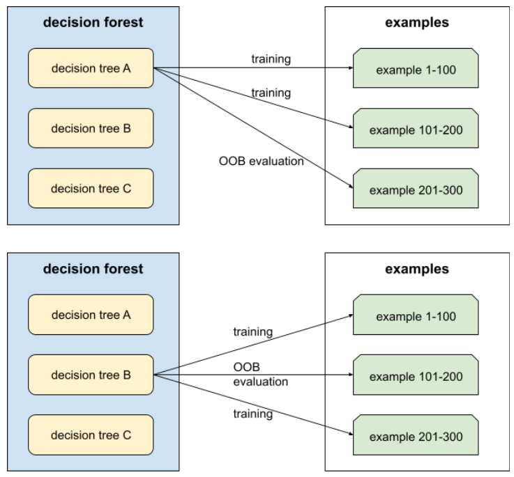
袋外评估是一种计算效率高且保守的交叉验证机制近似值。在交叉验证中,每个交叉验证轮次都会训练一个模型(例如,在 10 折交叉验证中会训练 10 个模型)。使用 OOB 评估时,系统会训练单个模型。由于 bagging 在训练期间会从每棵树中留出一些数据,因此 OOB 评估可以使用这些数据来近似交叉验证。
如需了解详情,请参阅决策森林课程中的袋外评估。
输出层
神经网络的“最终”层。输出层包含预测结果。
下图展示了一个小型深度神经网络,其中包含一个输入层、两个隐藏层和一个输出层:
过拟合
创建的模型与训练数据过于匹配,以致于模型无法根据新数据做出正确的预测。
正则化可以减少过拟合。 在庞大而多样的训练集上进行训练也有助于减少过拟合。
如需了解详情,请参阅机器学习速成课程中的过拟合。
过采样
在类别不平衡的数据集中重复使用少数类的示例,以创建更平衡的训练集。
例如,假设有一个二元分类问题,其中多数类与少数类的比率为 5,000:1。如果数据集包含 100 万个示例,那么少数类只包含大约 200 个示例,这可能不足以进行有效训练。为了克服这一不足,您可以多次对这 200 个示例进行过采样(重复使用),从而可能获得足够的示例来进行有效训练。
在过采样时,您需要注意避免过拟合。
与欠采样相对。
P
打包数据
一种更高效地存储数据的方法。
打包数据是指以压缩格式或以其他方式存储数据,以便更高效地访问数据。打包数据可最大限度地减少访问数据所需的内存和计算量,从而加快训练速度并提高模型推理效率。
打包数据通常与其他技术(例如数据增强和正则化)搭配使用,以进一步提高模型的性能。
PaLM
pandas
基于 numpy 构建的面向列的数据分析 API。 许多机器学习框架(包括 TensorFlow)都支持将 Pandas 数据结构作为输入。如需了解详情,请参阅 Pandas 文档。
参数
模型在训练期间学习的权重和偏差。例如,在线性回归模型中,参数包括以下公式中的偏差 (b) 和所有权重(w1、w2 等):
相比之下,超参数是您(或超参数调节服务)提供给模型的值。例如,学习速率就是一种超参数。
参数高效调优
一组用于比完全微调更高效地微调大型预训练语言模型 (PLM)的技术。与完全微调相比,参数高效调优通常会微调少得多的参数,但通常会生成性能与完全微调构建的大语言模型相当(或几乎相当)的大语言模型。
比较参数高效调优与以下方法的异同:
参数高效调优也称为参数高效微调。
参数服务器 (PS)
一种作业,负责在分布式环境中跟踪模型参数。
参数更新
在训练期间调整模型参数的操作,通常在单次梯度下降法迭代中进行。
偏导数
一种导数,其中除一个变量之外的所有变量都被视为常量。例如,f(x, y) 相对于 x 的偏导数是将 f 视为仅以 x 为变量的函数的导数(即保持 y 不变)。f 对 x 的偏导数仅关注 x 如何变化,而忽略公式中的所有其他变量。
参与偏差
与无反应误差的含义相同。请参阅选择性偏差。
划分策略
在参数服务器间分割变量的算法。
前 k 名的通过率 (pass@k)
一种用于确定大语言模型生成的代码(例如 Python)质量的指标。 更具体地说,Pass@k 表示在生成的 k 个代码块中,至少有一个代码块通过所有单元测试的可能性。
大语言模型通常难以针对复杂的编程问题生成优质代码。软件工程师通过提示大语言模型为同一问题生成多个 (k) 解决方案来应对这一问题。然后,软件工程师会针对单元测试对每个解决方案进行测试。通过率(在 k 处)的计算取决于单元测试的结果:
- 如果这些解决方案中的一个或多个通过了单元测试,则 LLM 通过了该代码生成挑战。
- 如果没有任何解决方案通过单元测试,则 LLM 未能通过该代码生成挑战。
通过率(在 k 处)的公式如下:
\[\text{pass at k} = \frac{\text{total number of passes}} {\text{total number of challenges}}\]
一般来说,k 值越高,pass@k 得分就越高;不过,k 值越高,所需的大语言模型和单元测试资源就越多。
Pathways Language Model (PaLM)
一种旧版模型,是 Gemini 模型的前身。
Pax
一种编程框架,旨在训练大规模神经网络 模型,这些模型非常庞大,以至于需要跨多个 TPU 加速器芯片 切片或 Pod。
Pax 基于 Flax 构建,而 Flax 基于 JAX 构建。
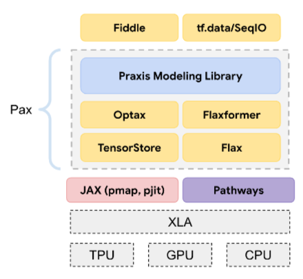
感知机
一种系统(硬件或软件),该系统先获取一个或多个输入值,接着对这些输入的加权和运行函数,然后计算单个输出值。在机器学习中,该函数通常是非线性函数,例如 ReLU、sigmoid 或 tanh。 例如,以下感知机依赖 S 型函数来处理三个输入值:
在下图中,感知机先获取三个输入,每个输入本身会经过权重的修改,然后才进入感知机:

性能
一个多含义术语,具有以下含义:
- 在软件工程中的标准含义。即:软件的运行速度有多快(或有多高效)?
- 在机器学习中的含义。在机器学习领域,性能旨在回答以下问题:模型的准确度有多高?即模型在预测方面的表现有多好?
排列变量重要性
一种变量重要性,用于评估在对特征值进行置换后模型预测误差的增加情况。排列变量重要性是一种与模型无关的指标。
困惑度
一种衡量指标,用于衡量模型能够多好地完成任务。 例如,假设您的任务是读取用户在手机键盘上输入的单词的前几个字母,并提供可能的补全字词列表。此任务的困惑度 P 大致是指您需要提供多少个猜测,才能使您的列表包含用户尝试输入的实际字词。
困惑度与交叉熵的关系如下:
流水线
机器学习算法周围的基础设施。流水线包括收集数据、将数据放入训练数据文件、训练一个或多个模型,以及将模型导出到生产环境。
如需了解详情,请参阅“管理机器学习项目”课程中的 ML 流水线。
流水线
一种模型并行处理形式,其中模型的处理分为连续的阶段,每个阶段在不同的设备上执行。当某个阶段处理一个批次时,前一个阶段可以处理下一个批次。
另请参阅分阶段训练。
pjit
一种 JAX 函数,用于拆分代码以在多个加速器芯片上运行。用户将一个函数传递给 pjit,该函数会返回一个具有等效语义的函数,但该函数会被编译为在多个设备(例如 GPU 或 TPU 核心)上运行的 XLA 计算。
pjit 使用户能够通过 SPMD 分区器对计算进行分片,而无需重写计算。
截至 2023 年 3 月,pjit 已与 jit 合并。如需了解详情,请参阅分布式数组和自动并行化。
plan-and-solve
一种智能体策略,模型先起草一个明确的多步计划,然后再尝试执行任何操作。
PLM
预训练语言模型的缩写。
插件
一种标准化、模块化的工具,可轻松附加到代理以扩展其功能。例如,GitHub 插件可让代理执行读取 GitHub 问题和创建拉取请求等操作。
pmap
一种 JAX 函数,可在多个底层硬件设备(CPU、GPU 或 TPU)上执行输入函数的副本,并使用不同的输入值。pmap 依赖于 SPMD。
政策
池化
将一个或多个由前面的卷积层创建的矩阵压缩为较小的矩阵。 池化通常涉及取池化区域中的最大值或平均值。例如,假设我们有以下 3x3 矩阵:
![3x3 矩阵 [[5,3,1], [8,2,5], [9,4,3]]。](https://developers.google.com/static/machine-learning/glossary/images/PoolingStart.svg?hl=zh-cn)
池化运算与卷积运算类似:将矩阵分割为多个切片,然后按步长逐个运行卷积运算。例如,假设池化运算以 1x1 的步长将卷积矩阵分割为 2x2 的切片。如下图所示,系统会执行四次池化操作。假设每个池化操作都会选择相应切片中的最大值:
![输入矩阵为 3x3,值如下:[[5,3,1], [8,2,5], [9,4,3]]。
输入矩阵的左上角 2x2 子矩阵为 [[5,3], [8,2]],因此左上角池化操作会生成值 8(即 5、3、8 和 2 中的最大值)。输入矩阵的右上角 2x2 子矩阵为 [[3,1], [2,5]],因此右上角池化运算会产生值 5。输入矩阵的左下角 2x2 子矩阵为 [[8,2], [9,4]],因此左下角池化操作会产生值 9。输入矩阵的右下角 2x2 子矩阵为 [[2,5], [4,3]],因此右下角池化操作会生成值 5。总而言之,池化操作会生成 2x2 矩阵 [[8,5], [9,5]]。](https://developers.google.com/static/machine-learning/glossary/images/PoolingConvolution.svg?hl=zh-cn)
池化有助于在输入矩阵中实现平移不变性。
用于视觉应用的池化更正式的名称是空间 pooling。时序应用通常将池化称为时序池化。在不太正式的场合,池化通常称为下采样。
位置编码
一种将序列中词法单元的位置信息添加到词法单元嵌入中的技术。Transformer 模型使用位置编码来更好地了解序列不同部分之间的关系。
位置编码的常见实现方式是使用正弦函数。(具体而言,正弦函数的频率和振幅由序列中令牌的位置决定。)这种技术使 Transformer 模型能够根据序列中不同部分的位置来学习关注这些部分。
正类别
您要测试的类。
例如,在癌症模型中,正类别可以是“肿瘤”。 在电子邮件分类模型中,正类别可以是“垃圾邮件”。
与负类别相对。
后处理
在模型运行后调整其输出。 后期处理可用于强制执行公平性限制,而无需修改模型本身。
例如,可以对二元分类模型应用后处理,方法是设置分类阈值,以通过检查真正例率对于某个属性的所有值是否相同,来维持该属性的机会均等。
后训练模型
一个宽泛定义的术语,通常是指经过一些后处理(例如以下一项或多项)的预训练模型:
PR AUC(PR 曲线下的面积)
通过绘制不同分类阈值的(召回率、精确率)点而获得的插值精确率-召回率曲线下的面积。
Praxis
Pax 的核心高性能机器学习库。Praxis 通常称为“Layer 库”。
Praxis 不仅包含 Layer 类的定义,还包含其大部分支持组件,包括:
Praxis 为 Model 类提供定义。
精确度
一种分类模型指标,可为您提供以下信息:
当模型预测为正类别时,预测正确的百分比是多少?
公式如下:
其中:
- 真正例是指模型正确预测了正类别。
- 假正例是指模型错误地预测了正类别。
例如,假设某个模型做出了 200 次正预测。在这 200 个正例预测中:
- 其中 150 个是真正例。
- 其中 50 个是假正例。
在此示例中:
如需了解详情,请参阅机器学习速成课程中的分类:准确率、召回率、精确率和相关指标。
前 k 名的精确率(precision@k)
用于评估排名(有序)商品列表的指标。 前 k 项的精确率是指该列表中的前 k 项中“相关”项所占的比例。具体来说:
\[\text{precision at k} = \frac{\text{relevant items in first k items of the list}} {\text{k}}\]
k 的值必须小于或等于返回列表的长度。 请注意,返回列表的长度不属于计算的一部分。
相关性通常是主观的;即使是专业的人工评估员也经常在哪些内容相关的问题上意见不一。
比较对象:
精确率与召回率曲线
预测
模型的输出。例如:
- 二元分类模型的预测结果要么是正类别,要么是负类别。
- 多类别分类模型的预测结果是一个类别。
- 线性回归模型的预测结果是一个数值。
预测偏差
预测性机器学习
任何标准(“经典”)机器学习系统。
“预测性机器学习”一词没有正式定义。相反,该术语用于区分不基于生成式 AI 的一类机器学习系统。
预测性平价
一种公平性指标,用于检查对于给定的分类模型,所考虑的子群组的精确率是否相等。
例如,如果某个预测大学录取情况的模型对小人国人和巨人国人的精确率相同,则该模型会满足“预测平等”这一条件。
预测性均等有时也称为预测率均等。
如需更详细地了解预测对等性,请参阅“公平性定义说明”(第 3.2.1 部分)。
预测性价格一致性
预测奇偶性的另一个名称。
预处理
在数据用于训练模型之前对其进行处理。预处理可以很简单,例如从英文文本语料库中移除未出现在英语词典中的字词;也可以很复杂,例如以尽可能消除与敏感属性相关联的属性的方式重新表达数据点。预处理有助于满足公平性限制条件。预训练模型
虽然此术语可以指任何经过训练的模型或经过训练的嵌入向量,但预训练模型现在通常是指经过训练的大语言模型或其他形式的经过训练的生成式 AI 模型。
预训练
在大型数据集上对模型进行初始训练。有些预训练模型是笨拙的巨人,通常必须通过额外的训练来改进。 例如,机器学习专家可能会使用庞大的文本数据集(例如维基百科中的所有英文网页)预训练大语言模型。预训练完成后,可以通过以下任一技术进一步优化生成的模型:
先验信念
在开始用数据进行训练之前,您对这些数据抱有的信念。 例如,L2 正则化依赖于这样一种先验信念:权重应该很小且以 0 为中心呈正态分布。
Pro
Gemini 模型,参数数量少于 Ultra,但多于 Nano。如需了解详情,请参阅 Gemini Pro。
概率
一般而言,任何根据可能性或几率做出决策的情况。LLM 是概率性系统,会根据概率生成回答中的下一个字词或句子。
如果温度相对较低,LLM 会选择概率较高的字词或句子。如果温度相对较高,LLM 会更具“创意”,有时会选择概率较低的字词或句子。
概率回归模型
一种回归模型,不仅使用每个特征的权重,还使用这些权重的不确定性。概率回归模型会生成预测以及相应预测的不确定性。例如,概率回归模型可能会生成 325 的预测值,标准差为 12。如需详细了解概率回归模型,请参阅 tensorflow.org 上的这个 Colab。
概率密度函数
一种用于确定具有确切特定值的数据样本的频次的函数。如果数据集的值是连续的浮点数,则很少会出现完全匹配的情况。不过,对概率密度函数从值 x 到值 y 进行积分,可得出介于 x 和 y 之间的数据样本的预期频次。
例如,假设有一个平均值为 200、标准差为 30 的正态分布。若要确定落在 211.4 到 218.7 范围内的数据样本的预期频次,您可以对正态分布的概率密度函数从 211.4 到 218.7 进行积分。
程序性记忆
在代理中,指如何做某事的知识。例如,智能体可能会形成有关如何搜索网络然后显示前三个网站的程序性记忆。
提示
作为输入内容输入到大语言模型中的任何文本,用于让模型以某种特定方式运作。提示可以短至一个短语,也可以任意长(例如,整本小说的文本)。提示可分为多种类别,包括下表所示的类别:
| 提示类别 | 示例 | 备注 |
|---|---|---|
| 问题 | 鸽子能飞多快? | |
| 指令 | 写一首关于套利的趣味小诗。 | 要求大语言模型执行某种操作的提示。 |
| 示例 | 将 Markdown 代码转换为 HTML。例如:
Markdown:* 列表项 HTML:<ul> <li>列表项</li> </ul> |
此示例提示中的第一句话是一条指令。 提示的其余部分是示例。 |
| 角色 | 向物理学博士解释为什么在机器学习训练中使用梯度下降法。 | 句子的第一部分是指令;“物理学博士”一词是角色部分。 |
| 供模型补全的部分输入 | 英国首相居住在 | 部分输入提示可以突然结束(如本例所示),也可以以下划线结尾。 |
生成式 AI 模型可以根据提示生成文本、代码、图片、嵌入、视频…几乎任何内容。
基于提示的学习
某些模型的一项功能,可让模型根据任意文本输入(提示)调整其行为。在典型的基于提示的学习范式中,大语言模型通过生成文本来响应提示。例如,假设用户输入了以下提示:
总结牛顿第三运动定律。
能够基于提示进行学习的模型并非专门经过训练来回答之前的提示。相反,模型“知道”很多关于物理学的事实、很多关于一般语言规则的知识,以及很多关于哪些答案通常有用的知识。这些知识足以提供(希望)有用的答案。其他人类反馈(例如“这个回答太复杂了”或“什么是反应?”)使一些基于提示的学习系统能够逐步提高回答的实用性。
提示链
将一个提示的输出用作另一个提示的输入。 从少到多提示是一种常见的提示链形式。
提示设计
与提示工程的含义相同。
提示工程
创建提示的艺术,这些提示可从大语言模型中引出所需的回答。人类执行提示工程。编写结构化良好的提示是确保从大语言模型获得有用回答的重要环节。提示工程取决于多种因素,包括:
提示设计是提示工程的同义词。
如需详细了解如何撰写有用的提示,请参阅提示设计简介。
提示集
用于评估大语言模型的一组提示。例如,下图显示了一个包含三个提示的提示集:
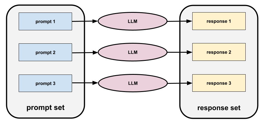
优秀的提示集包含足够“广泛”的提示,可用于全面评估大语言模型的安全性和实用性。
另请参阅回答集。
提示调优
一种参数高效调优机制,用于学习系统预先添加到实际提示中的“前缀”。
提示调优的一种变体(有时称为“前缀调优”)是在每个层前面添加前缀。相比之下,大多数提示调优仅向输入层添加前缀。
provenance
详细说明数字媒体内容如何创建或更改的数据。
代理(敏感属性)
用作敏感属性的替代属性。例如,个人的邮政编码可能会被用作其收入、种族或民族的代理变量。代理标签
用于逼近未在数据集内直接提供的标签的数据。
例如,假设您必须训练一个模型来预测员工压力水平。您的数据集包含许多预测性特征,但不包含名为 stress level 的标签。您毫不气馁,选择“工作场所事故”作为压力水平的代理标签。毕竟,压力过大的员工比心态平静的员工更容易发生事故。或者说,他们会这样做吗?或许,工作场所事故的发生率实际上会因多种原因而上升和下降。
再举一个例子,假设您希望将“是否下雨?”作为数据集的布尔型标签,但您的数据集不包含下雨数据。如果有照片,您能够以人们带着雨伞的照片作为“在下雨吗?”的代理标签。这是一个好的代理标签吗?可能,但某些文化背景的人可能更倾向于带伞防晒,而不是防雨。
代理标签通常并不完美。如果可以,请选择实际标签,而不是代理标签。不过,如果缺少实际标签,请非常谨慎地选择代理标签,选择最不糟糕的代理标签候选对象。
如需了解详情,请参阅机器学习速成课程中的数据集:标签。
纯函数
一种函数,其输出仅基于输入,且没有附带效应。具体来说,纯函数不会使用或更改任何全局状态,例如文件内容或函数外部的变量值。
纯函数可用于创建线程安全的代码,这在跨多个加速器芯片对模型代码进行分片时非常有用。
JAX 的函数转换方法要求输入函数是纯函数。
Q
Q 函数
在强化学习中,用于预测在状态下采取行动并遵循给定策略所获得的预期回报的函数。
Q 函数也称为状态-动作值函数。
Q-learning
在强化学习中,一种算法通过应用 Bellman 方程,使智能体能够学习 Markov 决策过程的最佳 Q 函数。马尔可夫决策过程可对环境进行建模。
分位数
分位数分桶中的每个分桶。
分位数分桶
将一个特征的值分发到桶中,使每个桶包含的样本数量相同(或几乎相同)。例如,下图将 44 个点分到 4 个桶中,每个桶包含 11 个点。为使图中每个分桶包含的点数相同,有些分桶对应的 x 值的跨度不同。

如需了解详情,请参阅机器学习速成课程中的数值数据:分箱。
量化
一个多含义术语,可用于以下任何一种情况:
- 对特定特征实现分位数分桶。
- 将数据转换为 0 和 1,以便更快地存储、训练和推理。与采用其他格式的数据相比,布尔数据对噪声和错误的稳健性更强,因此量化可以提高模型的正确性。 量化技术包括舍入、截断和分箱。
减少用于存储模型参数的位数。例如,假设模型的形参存储为 32 位浮点数。量化会将这些参数从 32 位转换为 4 位、8 位或 16 位。量化可减少以下方面:
- 计算、内存、磁盘和网络用量
- 推理预测的时间
- 功耗
不过,量化有时会降低模型预测的正确性。
队列
一种实现队列数据结构的 TensorFlow 操作。通常用于 I/O。
R
RAG
检索增强生成的缩写。
随机森林
一种决策树集成,其中每个决策树都使用特定的随机噪声进行训练,例如装袋。
随机森林是一种决策森林。
如需了解详情,请参阅决策森林课程中的随机森林。
随机政策
排序(序数)
在将类别从最高到最低进行分类的机器学习问题中,类别的顺序位置。例如,行为排序系统可以将狗狗的奖励从最高(牛排)到最低(枯萎的羽衣甘蓝)进行排序。
秩(张量)(rank (Tensor))
Tensor中的维数。例如,标量的秩为 0,向量的秩为 1,矩阵的秩为 2。
请勿与排序(序数)混淆。
排名
一种监督学习,其目标是对项目列表进行排序。
标注者
如需了解详情,请参阅机器学习速成课程中的分类数据:常见问题。
使用常识推理数据集 (ReCoRD) 进行阅读理解
用于评估 LLM 执行常识推理能力的数据集。 数据集中的每个示例都包含三个组成部分:
- 新闻报道中的一两个段落
- 一种查询,其中段落中明确或隐式标识的某个实体被遮盖。
- 答案(属于遮盖的实体的名称)
如需查看大量示例,请参阅 ReCoRD。
ReCoRD 是 SuperGLUE 集成模型的一个组成部分。
RealToxicityPrompts
包含一组可能包含有害内容的句子开头的数据集。使用此数据集评估 LLM 生成无毒文本以完成句子的能力。通常,您会使用 Perspective API 来确定 LLM 在此任务中的表现。
如需了解详情,请参阅RealToxicityPrompts:评估语言模型中的神经毒性退化。
reason
agentic loop 中的一个阶段,在此阶段,代理会确定要执行的操作。例如,代理可能会确定应发送特定的 API 请求。
召回
一种分类模型指标,可为您提供以下信息:
公式如下:
\[\text{Recall} = \frac{\text{true positives}} {\text{true positives} + \text{false negatives}} \]
其中:
- 真正例是指模型正确预测了正类别。
- 假负例是指模型错误地预测了负类别。
例如,假设您的模型对评估依据为正类别的样本进行了 200 次预测。在这 200 个预测中:
- 其中 180 个是真正例。
- 20 个为假负例。
在此示例中:
\[\text{Recall} = \frac{\text{180}} {\text{180} + \text{20}} = 0.9 \]
如需了解详情,请参阅分类:准确率、召回率、精确率和相关指标。
前 k 名召回率 (recall@k)
一种用于评估输出排名(有序)商品列表的系统的指标。 “前 k 项的召回率”是指在返回的相关项总数中,相应列表的前 k 项中相关项所占的比例。
\[\text{recall at k} = \frac{\text{relevant items in first k items of the list}} {\text{total number of relevant items in the list}}\]
与 k 处的精确率相对。
识别文本蕴涵关系 (RTE)
一个用于评估 LLM 是否能够确定假设是否可以从文本段落中得出(逻辑上)的数据集。RTE 评估中的每个示例都包含三个部分:
- 一段文字,通常来自新闻或维基百科文章
- 假设
- 正确答案(以下任一选项):
- True,表示假设可以从段落中推导出来
- False,表示假设无法从段落中得出
例如:
- 原文:欧元是欧盟的货币。
- 假设:法国使用欧元作为货币。
- 蕴涵:为 True,因为法国是欧盟的一部分。
RTE 是 SuperGLUE 集成模型的一个组成部分。
推荐系统
一种系统,从大型语料库为每位用户选择相对较小的所需推荐项集合。例如,视频推荐系统可能会从包含 100000 部视频的语料库推荐两部视频,为一位用户选择《卡萨布兰卡》和《旧欢新宠:费城故事》,而为另一位用户选择《神奇女侠》和《黑豹》。视频推荐系统可能会根据以下因素进行推荐:
- 类似用户评过分或观看过的影片。
- 类型、导演、演员、目标受众…
如需了解详情,请参阅推荐系统课程。
ReCoRD
Reading Comprehension with Commonsense Reasoning Dataset 的缩写。
修正线性单元 (ReLU)
一种激活函数,具有以下行为:
- 如果输入为负数或零,则输出为 0。
- 如果输入为正数,则输出等于输入。
例如:
- 如果输入为 -3,则输出为 0。
- 如果输入为 +3,则输出为 3.0。
以下是 ReLU 的图:
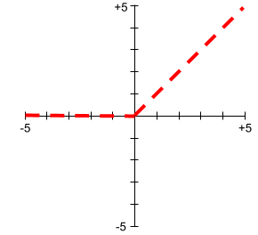
ReLU 是一种非常热门的激活函数。尽管 ReLU 的行为很简单,但它仍然能够让神经网络学习特征与标签之间的非线性关系。
循环神经网络
特意运行多次的神经网络,其中每次运行的部分结果会馈送到下一次运行。具体来说,上一次运行时隐藏层中的结果会作为下一次运行时相同隐藏层的部分输入。循环神经网络在评估序列时尤其有用,因此隐藏层可以根据神经网络在序列的前几部分上的前几次运行进行学习。
例如,下图显示了运行四次的循环神经网络。请注意,第一次运行时在隐藏层中学习的值将成为第二次运行时相同隐藏层的部分输入。同样,第二次运行时在隐藏层中学习的值将成为第三次运行时相同隐藏层的部分输入。通过这种方式,循环神经网络逐步训练和预测整个序列的含义,而不只是各个字词的含义。

参考文本
专家对提示的回答。例如,假设有以下提示:
将问题“What is your name?”从英语翻译成法语。
专家的回答可能是:
Comment vous appelez-vous?
各种指标(例如 ROUGE)用于衡量参考文本与机器学习模型生成的文本的匹配程度。
反思
一种用于提高智能体工作流质量的策略,即在将某一步骤的输出传递给下一步骤之前,先检查(反思)该输出。
检查者通常是生成回答的同一 LLM(不过也可能是其他 LLM)。生成回答的 LLM 如何才能公平地评判自己的回答?“诀窍”是让 LLM 处于批判性(反思性)思维模式。这个过程类似于作家先以创意的心态撰写初稿,然后切换到批判性思维模式进行编辑。
例如,假设有一个智能体工作流,其第一步是为咖啡杯创建文字。此步骤的提示可能如下所示:
您是创作者。生成幽默风趣且不超过 50 个字符的原创文字,适合印在咖啡杯上。
现在,假设有以下反思性提示:
您是咖啡饮用者。您会觉得上述回答幽默吗?
然后,工作流可能只会将获得高反思得分的文本传递到下一阶段。
回归模型
从非正式意义上讲,一种生成数值预测的模型。(相比之下,分类模型会生成类别预测结果。)例如,以下都是回归模型:
- 预测特定房屋价值(以欧元为单位)的模型,例如 423,000 欧元。
- 一种模型,用于预测特定树木的预期寿命(以年为单位),例如 23.2 年。
- 一种模型,用于预测未来 6 小时内某个城市将降雨的量(以英寸为单位),例如 0.18。
以下是两种常见的回归模型:
并非所有输出数值预测的模型都是回归模型。在某些情况下,数值预测实际上只是一个恰好具有数值类别名称的分类模型。例如,预测数值邮政编码的模型是分类模型,而不是回归模型。
正则化
任何可减少过拟合的机制。 常见的正则化类型包括:
- L1 正则化
- L2 正则化
- dropout 正规化
- 早停法(这不是正式的正则化方法,但可以有效限制过拟合)
正则化也可以定义为对模型复杂性的惩罚。
如需了解详情,请参阅机器学习速成课程中的过拟合:模型复杂性。
正则化率
一个数字,用于指定训练期间正则化的相对重要性。提高正则化率可减少过拟合,但可能会降低模型的预测能力。相反,降低或省略正则化率会增加过拟合。
如需了解详情,请参阅机器学习速成课程中的过拟合:L2 正则化。
强化学习 (RL)
一类算法,用于学习最佳策略,其目标是在与环境互动时最大限度地提高回报。例如,大多数游戏的最终奖励是胜利。 通过对最终带来胜利前的游戏走法序列和最终导致失败的序列进行评估,强化学习系统会变得擅长玩复杂的游戏。
基于人类反馈的强化学习 (RLHF)
使用人工评估者的反馈来提高模型回答的质量。例如,RLHF 机制可以要求用户使用 👍 或 👎 表情符号对模型回答的质量进行评分。然后,系统可以根据该反馈调整其未来的回答。
ReLU
修正线性单元的缩写。
回放缓冲区
在类似 DQN 的算法中,智能体用于存储状态转换以供经验回放使用的内存。
副本
训练集或模型的副本(或部分),通常存储在另一台机器上。例如,系统可以使用以下策略来实现数据并行:
- 将现有模型的副本放置在多台机器上。
- 向每个副本发送不同的训练集子集。
- 汇总 形参更新。
副本还可以指推理服务器的另一个副本。增加副本数量可以增加系统可同时处理的请求数量,但也会增加服务费用。
通报偏差
一种事实,即人们对操作、结果或属性进行描述的频率不能反映这些内容实际出现的频率或者某个属性在多大程度上是某类个体的特征。通报偏差可以影响机器学习系统从中学习规律的数据的构成。
例如,在书中,“laughed”比“breathed”更普遍。机器学习模型对书籍语料库中的“laughing”和“breathing”的相对频率进行评估后,可能会确定“laughing”比“breathing”更常见。
如需了解详情,请参阅机器学习速成课程中的公平性:偏差类型。
相同的矢量表示。
将数据映射到实用特征的过程。
重排序
推荐系统的最后阶段,在此期间,可能会根据其他(通常是非机器学习)算法,对已获得评分的推荐项重新评分。重排序会对在打分阶段生成的推荐项列表进行评估,然后采取以下操作:
- 消除用户已购买的推荐项。
- 提高较新推荐项的得分。
如需了解详情,请参阅推荐系统课程中的重排序。
Response
生成式 AI 模型推理出的文字、图片、音频或视频。换句话说,提示是生成式 AI 模型的输入,而回答是输出。
回答集
检索增强生成 (RAG)
一种技术,利用模型训练后检索到的知识源进行接地,以改善大语言模型 (LLM) 的输出质量。RAG 通过为经过训练的 LLM 提供从可信知识库或文档中检索到的信息,提高了 LLM 回答的准确性。
使用检索增强生成的常见动机包括:
- 提高模型生成回答的事实准确性。
- 让模型能够访问其未经训练的知识。
- 更改模型使用的知识。
- 使模型能够引用来源。
例如,假设某个化学应用使用 PaLM API 生成与用户查询相关的摘要。当应用的后端收到查询时,后端会执行以下操作:
- 搜索(“检索”)与用户查询相关的数据。
- 将相关化学数据附加(“扩充”)到用户查询中。
- 指示 LLM 根据附加的数据创建摘要。
回车键
在强化学习中,给定某个政策和某个状态,回报是指智能体在从状态开始到情节结束期间遵循政策时预期会收到的所有奖励之和。智能体会根据获得奖励所需的状态转换来对奖励进行折扣,从而考虑预期奖励的延迟性。
因此,如果折扣率为 \(\gamma\),且 \(r_0, \ldots, r_{N}\)表示直至剧集结束时的奖励,则回报计算如下:
奖励
岭正则化
与 L2 正则化的同义词。岭正则化一词更常用于纯粹的统计学领域,而 L2 正则化更常用于机器学习中。
RNN
循环神经网络的缩写。
ROC(接收者操作特征)曲线
ROC 曲线的形状表明了二元分类模型区分正类别和负类别的能力。例如,假设某个二元分类模型能够完美区分所有负类别和所有正类别:
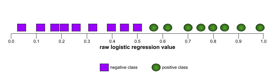
上述模型的 ROC 曲线如下所示:
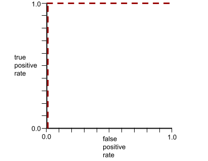
相比之下,下图绘制了一个糟糕模型的原始逻辑回归值,该模型根本无法区分负类和正类:
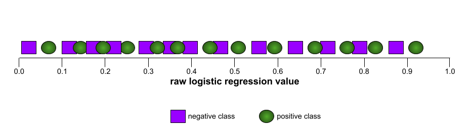
相应模型的 ROC 曲线如下所示:
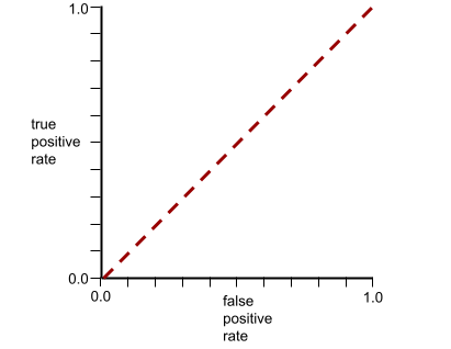
与此同时,在现实世界中,大多数二元分类模型都会在一定程度上区分正类别和负类别,但通常不会完全区分。因此,典型的 ROC 曲线介于这两个极端之间:
从理论上讲,ROC 曲线上最接近 (0.0,1.0) 的点可确定理想的分类阈值。不过,还有一些其他实际问题会影响理想分类阈值的选择。例如,假负例造成的损失可能远高于假正例。
一种名为 AUC 的数值指标可将 ROC 曲线汇总为单个浮点值。
角色提示
一种提示,通常以代词“你”开头,用于告知生成式 AI 模型在生成回答时假装成特定的人或扮演特定的角色。 角色提示可帮助生成式 AI 模型进入正确的“思维模式”,从而生成更有用的回答。例如,根据您希望获得的回答类型,以下任何角色提示都可能适用:
您拥有计算机科学博士学位。
您是一名软件工程师,喜欢耐心地向新学程序设计的学生讲解 Python。
您是一位行动英雄,拥有非常专业的编程技能。 向我保证,您会在 Python 列表中找到特定项。
root
决策树中的起始节点(第一个条件)。按照惯例,图表会将根放在决策树的顶部。例如:
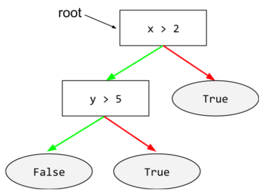
根目录
您指定的目录,用于托管多个模型的 TensorFlow 检查点和事件文件的子目录。
均方根误差 (RMSE)
均方误差的平方根。
旋转不变性
在图像分类问题中,即使图像的方向发生变化,算法也能成功对图像进行分类的能力。例如,无论网球拍是向上、侧向还是向下,该算法仍然可以识别它。请注意,并非总是需要旋转不变性;例如,倒置的“9”不应分类为“9”。
ROUGE(以召回率为导向的摘要评估研究)
用于评估自动摘要和机器翻译模型的一系列指标。 ROUGE 指标用于确定参考文本与机器学习模型生成的文本之间的重叠程度。ROUGE 系列中的每个成员都以不同的方式衡量重叠程度。ROUGE 得分越高,表示参考文本与生成的文本之间的相似度越高;ROUGE 得分越低,表示参考文本与生成的文本之间的相似度越低。
每个 ROUGE 系列成员通常会生成以下指标:
- 精确率
- 召回率
- F1
如需了解详情和示例,请参阅:
ROUGE-L
ROUGE 系列的成员,侧重于参考文本和生成文本中最长公共子序列的长度。以下公式用于计算 ROUGE-L 的召回率和精确率:
然后,您可以使用 F1 将 ROUGE-L 召回率和 ROUGE-L 精确率汇总为一个指标:
ROUGE-L 会忽略参考文本和生成文本中的所有换行符,因此最长公共子序列可能会跨越多个句子。如果参考文本和生成的文本包含多个句子,那么通常最好使用 ROUGE-L 的一种变体,即 ROUGE-Lsum。ROUGE-Lsum 会确定段落中每个句子的最长公共子序列,然后计算这些最长公共子序列的平均值。
ROUGE-N
ROUGE 系列中的一组指标,用于比较参考文本和生成文本中特定大小的共享 N 元语法。例如:
- ROUGE-1 用于衡量参考文本和生成文本中共享的 token 数量。
- ROUGE-2 用于衡量参考文本和生成的文本中共享的二元语法(2-gram)数量。
- ROUGE-3 用于衡量参考文本和生成的文本中共享的三元语法(3-gram)数量。
您可以使用以下公式计算任何 ROUGE-N 成员的 ROUGE-N 召回率和 ROUGE-N 精确率:
然后,您可以使用 F1 将 ROUGE-N 召回率和 ROUGE-N 精确率汇总为一个指标:
ROUGE-S
一种宽松形式的 ROUGE-N,可实现 skip-gram 匹配。也就是说,ROUGE-N 只会统计完全匹配的 N 元语法,而 ROUGE-S 还会统计被一个或多个字词分隔的 N 元语法。例如,应该考虑以下事项:
计算 ROUGE-N 时,二元语法“白云”与“白色滚滚的云”不匹配。不过,在计算 ROUGE-S 时,白云与白色的滚滚云海相匹配。
路由器代理
一种对用户查询进行分类,然后调用最合适的代理来处理该查询的代理。
R 平方
一种回归指标,用于指示标签的变异中有多少是由单个特征或一个特征集造成的。R 平方是介于 0 和 1 之间的值,您可以按如下方式解读:
- R 平方值为 0 表示标签的任何变异都不是由特征集造成的。
- R 平方值为 1 表示标签的所有变异均由特征集导致。
- 介于 0 和 1 之间的 R 平方值表示标签的变化在多大程度上可以通过特定特征或特征集来预测。例如,R 平方值为 0.10 表示标签中 10% 的方差是由特征集造成的;R 平方值为 0.20 表示 20% 的方差是由特征集造成的,依此类推。
RTE
识别文本蕴涵的缩写。
S
采样偏差
请参阅选择性偏差。
放回抽样
一种从一组候选商品中挑选商品的方法,其中同一商品可以多次被选中。“有放回”是指每次选择后,所选项目都会返回到候选项目池中。相反的方法是不放回抽样,这意味着候选商品只能被选中一次。
例如,假设有以下水果集:
fruit = {kiwi, apple, pear, fig, cherry, lime, mango}假设系统随机选择 fig 作为第一个商品。如果采用放回抽样,系统会从以下集合中选择第二个项:
fruit = {kiwi, apple, pear, fig, cherry, lime, mango}是的,这与之前的设置相同,因此系统可能会再次选择 fig。
如果使用不放回抽样,一旦选中某个样本,就无法再次选中该样本。例如,如果系统随机选择 fig 作为第一个样本,则不能再次选择 fig。因此,系统会从以下(缩减的)集合中选择第二个样本:
fruit = {kiwi, apple, pear, cherry, lime, mango}SavedModel
保存和恢复 TensorFlow 模型时建议使用的格式。SavedModel 是一种独立于语言且可恢复的序列化格式,使较高级别的系统和工具可以创建、使用和转换 TensorFlow 模型。
如需完整的详细信息,请参阅《TensorFlow 编程人员指南》中的保存和恢复部分。
实惠
一种 TensorFlow 对象,负责保存模型检查点。
标量
可表示为秩为 0 的张量的单个数字或单个字符串。例如,以下每行代码都会在 TensorFlow 中创建一个标量:
breed = tf.Variable("poodle", tf.string)
temperature = tf.Variable(27, tf.int16)
precision = tf.Variable(0.982375101275, tf.float64)
扩缩
用于调整标签、特征值或两者的范围的任何数学转换或技术。某些形式的缩放对于归一化等转换非常有用。
机器学习中常用的缩放形式包括:
- 线性缩放,通常使用减法和除法的组合将原始值替换为介于 -1 和 +1 之间或介于 0 和 1 之间的数字。
- 对数缩放,即将原始值替换为其对数。
- Z-score 归一化,即将原始值替换为表示该特征与平均值之间相差的标准差数量的浮点值。
scikit-learn
一个热门的开源机器学习平台。请访问 scikit-learn.org。
评分
推荐系统的一部分,用于为候选集生成阶段生成的每个推荐项提供价值或排名。
选择性偏差
由于选择过程在数据中观察到的样本和未观察到的样本之间产生系统差异,因此根据抽样数据得出的结论存在误差。存在以下形式的选择性偏差:
- 覆盖偏差:数据集所代表的群体与机器学习模型要进行预测的群体不符。
- 采样偏差:数据不是从目标群体中随机收集的。
- 无反应误差(也称为参与偏差):某些群体中的用户以不同于其他群体中的用户的比率选择不参加调查问卷。
例如,假设您要创建一个机器学习模型来预测人们对电影的满意程度。为了收集训练数据,您向上映该电影的影院第一排的每个人发一份调查问卷。不假思索地话,这听起来像是收集数据集的合理方式,但是,这种数据收集方式可能会引入以下形式的选择性偏差:
- 覆盖偏差:通过从选择观看电影的人群中采样,您的模型预测可能不会泛化到那些对电影的兴趣尚未到达观看地步的人。
- 采样偏差:您仅对第一排的观众进行采样,而不是从预期群体(影院中的所有观众)进行随机采样。坐在第一排的观众可能比坐在其他排的观众对电影更感兴趣。
- 无反应误差:通常,相比具有温和观点的人,具有强烈观点的人倾向于更频繁地回答可选调查问卷。由于电影调查问卷是可选的,因此回复更有可能形成双峰分布,而不是正态(钟形)分布。
自注意力(也称为自注意力层)
一种神经网络层,可将嵌入序列(例如,令牌嵌入)转换为另一个嵌入序列。输出序列中的每个嵌入内容都是通过注意力机制整合输入序列元素中的信息来构建的。
自注意力中的“自”是指序列关注自身,而不是其他上下文。自注意力机制是 Transformer 的主要构建块之一,它使用字典查找术语,例如“查询”“键”和“值”。
自注意力层从一系列输入表示开始,每个字词对应一个输入表示。字词的输入表示可以是简单的嵌入。对于输入序列中的每个字词,网络会评估该字词与整个字词序列中每个元素的相关性。相关性得分决定了字词的最终表示形式在多大程度上纳入其他字词的表示形式。
例如,请看以下句子:
这只动物太累了,所以没有过马路。
下图(来自《Transformer:一种用于语言理解的新型神经网络架构》)显示了代词 it 的自注意力层注意力模式,其中每条线的深浅程度表示每个字词对表示法的贡献程度:
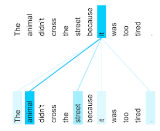
自注意力层会突出显示与“it”相关的字词。在这种情况下,注意力层已学会突出显示它可能指代的字词,并为动物分配最高权重。
对于包含 n 个令牌的序列,自注意力机制会分别在序列中的每个位置对嵌入序列进行 n 次转换。
自我修正
智能体检测自身输出中错误的能力,以及尝试不同方法的能力。
自监督式学习
一类技术,通过从无标签样本创建替代标签,将非监督式机器学习问题转换为监督式机器学习问题。
一些基于 Transformer 的模型(例如 BERT)使用自监督式学习。
自监督训练是一种半监督式学习方法。
自训练
一种 自监督学习的变体,在满足以下所有条件时特别有用:
自训练通过迭代执行以下两个步骤来运行,直到模型不再改进:
- 使用监督式机器学习基于有标签的示例训练模型。
- 使用第 1 步中创建的模型对无标签示例生成预测(标签),并将置信度高的示例移至有标签示例中,并附上预测的标签。
请注意,第 2 步的每次迭代都会为第 1 步添加更多带标签的示例以供训练。
语义记忆
LLM 在训练结束时拥有的信息。例如,语义记忆包括对语法、词汇以及明确训练的事实的出色知识。
语义记忆不包括从检索增强生成中收集的信息。
将语义记忆与情景记忆进行对比。
半监督式学习
基于部分训练示例有标签而其他训练示例没有标签的数据来训练模型。半监督式学习的一种方法是推断无标签样本的标签,然后根据推断出的标签进行训练,以创建新模型。如果获得有标签样本需要高昂的成本,而无标签样本则有很多,那么半监督式学习将非常有用。
自训练是半监督式学习的一种方法。
敏感属性
由于法律、道德、社会或个人原因,可能会受到特别关注的人类属性。情感分析
使用统计算法或机器学习算法确定群体对某个服务、产品、组织或主题的整体态度(积极或消极)。例如,使用自然语言理解,这种算法会通过对某大学课程的文字反馈进行情感分析,从而确定学生在多大程度上普遍喜欢或不喜欢该课程。
如需了解详情,请参阅文本分类指南。
序列模型
输入具有序列依赖性的模型。例如,根据之前观看过的一系列视频对观看的下一个视频进行预测。
序列到序列任务
一种将输入序列(包含 个词法单元)转换为输出词法单元序列的任务。例如,两种常见的序列到序列任务是:
- 翻译人员:
- 输入序列示例:“我爱你。”
- 输出序列示例:“Je t'aime.”
- 问答:
- 输入序列示例:“我在纽约市需要用车吗?”
- 输出序列示例:“No. Keep your car at home.”
人份
将训练好的模型部署上线,以便通过在线推理或离线推理提供预测结果的过程。
形状(张量)
张量的每个维度中的元素数量。形状以整数列表表示。例如,以下二维张量的形状为 [3,4]:
[[5, 7, 6, 4],
 [2, 9, 4, 8],
 [3, 6, 5, 1]]
TensorFlow 使用行优先(C 样式)格式来表示维度顺序,因此 TensorFlow 中的形状为 [3,4] 而不是 [4,3]。换句话说,在二维 TensorFlow 张量中,形状为 [行数、列数]。
静态形状是指在编译时已知的张量形状。
动态形状在编译时是未知的,因此取决于运行时数据。此张量在 TensorFlow 中可能以占位维度表示,如 [3, ?] 中所示。
分片
训练集或模型的逻辑划分。通常,某个进程会通过将示例或参数划分为(通常)大小相等的块来创建分片。然后,每个分片都会分配给不同的机器。
对模型进行分片称为模型并行处理;对数据进行分片称为数据并行处理。
收缩
梯度提升中的超参数,用于控制过拟合。梯度提升中的收缩率类似于梯度下降法中的学习速率。收缩率是介于 0.0 到 1.0 之间的小数值。与较大的收缩值相比,较小的收缩值可更有效地减少过拟合。
并排评估
通过判断两个模型对同一提示的回答来比较这两个模型的质量。例如,假设向两个不同的模型提供以下提示:
生成一张可爱的小狗玩三个球的图片。
在并排评估中,评估人员会选择哪张图片“更好”(更准确?更美观?更可爱?)。
S 型函数
一种数学函数,可将输入值“压缩”到有限的范围内,通常为 0 到 1 或 -1 到 +1。也就是说,您可以向 sigmoid 函数传递任何数字(2、100 万、负 10 亿,等等),输出结果仍会在限定范围内。 Sigmoid 激活函数的图如下所示:
S 型函数在机器学习中有多种用途,包括:
相似度度量
在聚类算法中,用于确定任何两种样本相似程度的指标。
单程序 / 多数据 (SPMD)
一种并行处理技术,可在不同设备上并行运行相同的计算,但使用不同的输入数据。SPMD 的目标是更快地获得结果。这是最常见的并行编程风格。
缩放不变性
在图像分类问题中,即使图像大小发生变化,算法也能成功对图像进行分类。例如,无论猫的像素数为 200 万还是 20 万,该算法仍然可以识别出猫。请注意,即使是最好的图片分类算法,在缩放不变性方面也仍存在实际限制。例如,对于仅以 20 像素呈现的猫图像,算法(或人)不可能正确对其进行分类。
如需了解详情,请参阅聚类分析课程。
粗略分析
在非监督式机器学习中,一类算法针对样本执行初步相似性分析。粗略分析算法使用 局部敏感哈希函数确定有可能相似的点,然后将这些点分组到桶中。
粗略分析减少了计算大型数据集相似性所需的计算量。我们仅计算每个桶中的每对点的相似性,而不是计算数据集内每对样本的相似性。
skip-gram
一种 n 元语法,可能会省略(或“跳过”)原始上下文中的字词,这意味着 N 个字词最初可能并不相邻。更准确地说,“k-skip-n-gram”是指最多可跳过 k 个字的 n-gram。
例如,“the quick brown fox”具有以下可能的 2-gram:
- "the quick"
- “quick brown”
- “brown fox”
“1-skip-2-gram”是指两个字词之间最多间隔 1 个字词。因此,“the quick brown fox”具有以下 1-skip 2-gram:
- “the brown”
- “quick fox”
此外,所有 2 元语法也都是 1-skip-2-gram,因为跳过的字词数可能少于一个。
Skip-gram 有助于了解单词周围的更多上下文。 在示例中,“fox”在 1-skip-2-gram 集中直接与“quick”相关联,但在 2-gram 集中并非如此。
Skip-gram 有助于训练字词嵌入模型。
softmax
一种函数,用于确定多类别分类模型中每个可能类别的概率。这些概率之和正好为 1.0。例如,下表显示了 softmax 如何分布各种概率:
| 图片是... | Probability |
|---|---|
| 狗 | 0.85 |
| 猫 | .13 |
| 马 | .02 |
Softmax 也称为完整 Softmax。
与候选采样相对。
如需了解详情,请参阅机器学习速成课程中的神经网络:多类别分类。
软提示调优
一种用于针对特定任务调整大语言模型的技术,无需资源密集型微调。与重新训练模型中的所有权重不同,软提示调优会自动调整提示,以实现相同的目标。
在给定文本提示的情况下,软提示调整通常会将额外的令牌嵌入附加到提示中,并使用反向传播来优化输入。
“硬”提示包含实际的令牌,而不是令牌嵌入。
稀疏特征
一种值主要为零或为空的特征。 例如,包含一个 1 值和一百万个 0 值的特征就是稀疏特征。相比之下,密集特征的值大多不为零或为空。
在机器学习中,出人意料的是,有大量特征是稀疏特征。分类特征通常是稀疏特征。例如,在森林中可能存在的 300 种树木中,单个示例可能仅标识出枫树。或者,在视频库中数百万个可能的视频中,一个示例可能仅标识“卡萨布兰卡”。
在模型中,您通常使用独热编码来表示稀疏特征。如果独热编码很大,您可以在独热编码之上放置一个嵌入层,以提高效率。
稀疏表示法
仅存储稀疏特征中非零元素的位置。
例如,假设某个名为 species 的分类特征用于标识特定森林中的 36 种树木。进一步假设每个示例仅标识一个物种。
您可以使用 one-hot 向量来表示每个示例中的树种。一个独热向量将包含一个 1(用于表示该示例中的特定树种)和 35 个 0(用于表示该示例中不存在的 35 个树种)。因此,maple 的独热表示法可能如下所示:
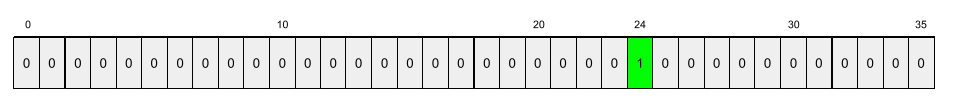
或者,稀疏表示法只会标识特定物种的位置。如果 maple 位于位置 24,则 maple 的稀疏表示法将非常简单:
24
请注意,稀疏表示法比 one-hot 表示法紧凑得多。
点击此图标可查看一个稍复杂的示例。
假设模型中的每个示例都必须表示英语句子中的字词(但不必表示这些字词的顺序)。 英语大约有 17 万个单词,因此英语是一个具有大约 17 万个元素的类别型特征。大多数英语句子只使用这 17 万个字词中极小的一部分,因此单个示例中的字词集几乎肯定是稀疏数据。
请看以下句子:
My dog is a great dog
您可以使用 one-hot 向量的变体来表示此句子中的字词。在此变体中,向量中的多个单元格可以包含非零值。此外,在此变体中,一个细胞可以包含除 1 以外的整数。虽然“my”“is”“a”和“great”这几个字词在句子中只出现一次,但“dog”一词出现了两次。使用这种单热向量变体来表示此句子中的字词会生成以下 17 万元素向量:
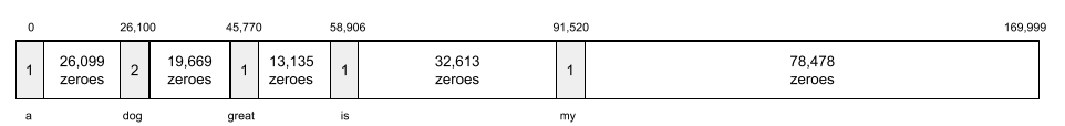
同一句子的稀疏表示法如下所示:
0: 1
26100: 2
45770: 1
58906: 1
91520: 1
如需了解详情,请参阅机器学习速成课程中的处理分类数据。
稀疏向量
稀疏性
向量或矩阵中设置为零(或 null)的元素数量除以该向量或矩阵中的条目总数。例如,假设有一个包含 100 个元素的矩阵,其中 98 个单元格包含零。稀疏度的计算方式如下:
特征稀疏度是指特征向量的稀疏度;模型稀疏度是指模型权重的稀疏度。
空间 pooling
请参阅 pooling。
规范化编码
以人类语言(例如英语)编写和维护描述软件的文件的过程。然后,您可以让生成式 AI 模型或其他软件工程师创建符合该描述的软件。
自动生成的代码通常需要迭代。在规范化编码中,您需要迭代说明文件。相比之下,在对话式编码中,您可以在提示框内进行迭代。在实践中,自动代码生成有时会涉及规范化编码和对话式编码的组合。
拆分
分割器
在训练决策树时,负责在每个节点上找到最佳条件的例程(和算法)。
SPMD
单程序 / 多数据的缩写。
SQuAD
斯坦福问答数据集的英文缩写,该数据集在论文《SQuAD:用于机器理解文本的 10 万多个问题》中进行了介绍。此数据集中的问题来自针对维基百科文章提出问题的用户。SQuAD 中的某些问题有答案,但其他问题故意没有答案。因此,您可以使用 SQuAD 来评估 LLM 在以下两方面的能力:
- 回答可以回答的问题。
- 确定无法回答的问题。
完全匹配与 F1 结合使用是根据 SQuAD 评估 LLM 的最常用指标。
平方合页损失函数
合页损失函数的平方。与常规合页损失函数相比,平方合页损失函数对离群值的惩罚更严厉。
平方损失函数
与 L2 损失的含义相同。
分阶段训练
一种以一系列离散阶段训练模型的策略。目标可以是加快训练过程,也可以是实现更好的模型质量。
下图展示了渐进式堆叠方法:
- 阶段 1 包含 3 个隐藏层,阶段 2 包含 6 个隐藏层,阶段 3 包含 12 个隐藏层。
- 第 2 阶段开始使用第 1 阶段 3 个隐藏层中学习到的权重进行训练。第 3 阶段开始使用第 2 阶段 6 个隐藏层中学习到的权重进行训练。
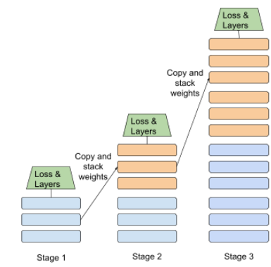
另请参阅流水线。
州
在强化学习中,用于描述环境当前配置的参数值,智能体使用这些参数值来选择行动。
状态-动作值函数
与 Q 函数的含义相同。
状态机代理
工作流受严格规则约束的代理。状态机代理通常比自主代理犯的错误更少,但无法灵活应对超出其限制的情况。
静态
一次性完成,而不是持续进行。 “静态”和“离线”这两个术语是同义词。 以下是机器学习中静态和离线的常见用途:
- 静态模型(或离线模型)是一种只训练一次,然后使用一段时间的模型。
- 静态训练(或离线训练)是指训练静态模型的过程。
- 静态推理(或离线推理)是指模型一次生成一批预测结果的过程。
与动态相对。
静态推理
与离线推理的含义相同。
平稳性
一种在一个或多个维度(通常是时间)上值保持不变的特征。 例如,如果某个特征在 2021 年和 2023 年的值大致相同,则该特征表现出平稳性。
在现实世界中,很少有特征表现出平稳性。即使是与稳定性同义的特征(例如海平面)也会随时间变化。
与非平稳性相对。
步骤
一次前向传递和一次后向传递,针对一个批次。
如需详细了解前向传递和后向传递,请参阅反向传播。
步长
与学习速率的含义相同。
随机梯度下降法 (SGD)
一种梯度下降法算法,其中批次大小为 1。换句话说,SGD 会基于从训练集中随机均匀选择的单个样本进行训练。
如需了解详情,请参阅机器学习速成课程中的线性回归:超参数。
步长
在卷积运算或池化中,下一系列输入切片的每个维度中的增量。例如,以下动画演示了卷积运算期间的 (1,1) 步长。因此,下一个输入切片从上一个输入切片右侧的一个位置开始。当操作到达右边缘时,下一个切片会一直向左移动,但会向下移动一个位置。
上例展示了二维步长。如果输入矩阵为三维,那么步长也将是三维。
结构风险最小化 (SRM)
一种平衡以下两个目标的算法:
- 需要构建最具预测性的模型(例如损失最低)。
- 需要使模型尽可能简单(例如强大的正则化)。
例如,旨在将基于训练集的损失和正则化降至最低的函数就是一种结构风险最小化算法。
与经验风险最小化相对。
分代理
一种由管理代理调用的专业化、专注型模型,用于处理较大问题中的特定子集。 子代理的动作空间通常比代理窄。
下采样
请参阅 pooling。
子词令牌
例如,“itemize”这样的字词可能会被拆分为“item”(词根)和“ize”(后缀),每个部分都由自己的令牌表示。将不常见的字词拆分为此类称为子字的片段,可让语言模型处理字词中更常见的组成部分,例如前缀和后缀。
相反,“going”等常用字词可能不会被拆分,而是由单个令牌表示。
摘要
在 TensorFlow 中的某一步计算出的一个值或一组值,通常用于在训练期间跟踪模型指标。
SuperGLUE
用于评估 LLM 理解和生成文本的整体能力的数据集集成。集成包含以下数据集:
- 布尔值问题 (BoolQ)
- CommitmentBank (CB)
- 合理替代方案选择 (COPA)
- 多句子阅读理解 (MultiRC)
- ReCoRD:基于常识推理的阅读理解数据集
- 识别文本蕴涵关系 (RTE)
- 上下文中的字词 (WiC)
- Winograd Schema Challenge (WSC)
如需了解详情,请参阅SuperGLUE:通用语言理解系统更具粘性的基准。
监督式机器学习
根据特征及其对应的标签训练模型。监督式机器学习类似于通过研究一系列问题及其对应的答案来学习某个知识。在掌握问题与答案之间的映射关系后,学生便可以回答同一主题的新问题(从未见过的问题)。
与非监督式机器学习相对。
如需了解详情,请参阅“机器学习简介”课程中的监督式学习。
合成特征
一种特征,不在输入特征之列,而是从一个或多个输入特征组装而来。用于创建合成特征的方法包括:
- 对连续特征进行分桶,以分为多个区间分箱。
- 创建特征组合。
- 将一个特征值与其他特征值或其本身相乘(或相除)。例如,如果
a和b是输入特征,则以下是合成特征的示例:- ab
- a2
- 将超越函数应用于要素值。例如,如果
c是输入特征,则以下是合成特征的示例:- sin(c)
- ln(c)
T
T5
Google AI 于 2020 年推出的文生文迁移学习 模型。T5 是一种基于 Transformer 架构的编码器-解码器模型,经过极大型数据集的训练。它在各种自然语言处理任务(例如生成文本、翻译语言和以对话方式回答问题)方面表现出色。
T5 的名称源自“文生文 Transfer Transformer”中的五个字母 T。
T5X
一个开源机器学习框架,旨在构建和训练大规模自然语言处理 (NLP) 模型。T5 是在 T5X 代码库(基于 JAX 和 Flax 构建)上实现的。
表格 Q-learning
在强化学习中,通过使用表格存储每个状态和动作组合的 Q 函数来实现 Q 学习。
目标
与标签的同义词。
目标网络
在深度 Q 学习中,神经网络是主要神经网络的稳定近似值,其中主要神经网络实现 Q 函数或策略。然后,您可以根据目标网络预测的 Q 值来训练主网络。因此,您可以防止主网络根据自身预测的 Q 值进行训练时出现的反馈循环。避免这种反馈可提高训练稳定性。
任务
可以使用机器学习技术解决的问题,例如:
任务分解
将大目标分解为可执行的原子步骤。 智能体通过执行任务分解来处理某些问题。
温度
一种超参数,用于控制模型输出的随机程度。温度越高,输出就越随机;温度越低,输出就越不随机。
选择最佳温度取决于具体的应用和/或字符串值。
时态数据
在不同时间点记录的数据。例如,一年中每天记录的冬季外套销售数据就是时态数据。
Tensor
TensorFlow 程序中的主要数据结构。张量是 N 维(其中 N 可能非常大)数据结构,最常见的是标量、向量或矩阵。张量的元素可以包含整数值、浮点值或字符串值。
TensorBoard
一个信息中心,用于显示在执行一个或多个 TensorFlow 程序期间保存的总结信息。
TensorFlow
一个大型的分布式机器学习平台。该术语还指 TensorFlow 堆栈中的基础 API 层,它支持对数据流图进行一般计算。
虽然 TensorFlow 主要用于机器学习,但您也可以将 TensorFlow 用于需要使用数据流图进行数值计算的非机器学习任务。
TensorFlow Playground
一款程序,用于可视化不同的超参数对模型(主要是神经网络)训练的影响。 如需试用 TensorFlow Playground,请前往 http://playground.tensorflow.org。
TensorFlow Serving
一个平台,用于将训练过的模型部署到生产环境。
张量处理单元 (TPU)
一种应用专用集成电路 (ASIC),用于优化机器学习工作负载的性能。这些 ASIC 作为 TPU 设备上的多个 TPU 芯片进行部署。
张量的阶
请参阅秩(张量)。
张量形状
Tensor在各种维度中包含的元素数。
例如,一个 [5, 10] 张量在一个维度上的形状为 5,在另一个维度上的形状为 10。
张量大小
Tensor包含的标量总数。例如,[5, 10] 张量的大小为 50。
TensorStore
用于高效读取和写入大型多维数组的库。
终止条件
在代理型 AI 中,预定义的标准用于告知代理停止迭代。例如,以下是一些可能的终止条件:
- 代理已成功完成目标。
- 智能体无法再使用任何资源。
- human-in-the-loop系统检测到问题。
在强化学习中,用于确定episode何时结束的条件,例如智能体何时达到特定状态或超过状态转换的阈值数量。例如,在井字棋(也称为圈叉棋)中,当玩家标记三个连续的空格或所有空格都被标记时,一集就会结束。
test
测试损失
表示模型针对测试集的损失的指标。在构建模型时,您通常会尝试最大限度地减少测试损失。这是因为,与较低的训练损失或较低的验证损失相比,较低的测试损失是更强的质量信号。
测试损失与训练损失或验证损失之间的差距过大有时表明您需要提高正则化率。
测试集
传统上,您需要将数据集中的示例划分为以下三个不同的子集:
数据集中的每个示例都应仅属于上述子集之一。 例如,单个样本不应同时属于训练集和测试集。
训练集和验证集都与模型训练密切相关。由于测试集仅与训练间接相关联,因此与训练损失或验证损失相比,测试损失是一种偏差更小、质量更高的指标。
如需了解详情,请参阅机器学习速成课程中的数据集:划分原始数据集。
文本 span
与文本字符串的特定子部分相关联的数组索引范围。例如,Python 字符串 s="Be good now" 中的字词 good 占据了从 3 到 6 的文本范围。
tf.Example
一种标准 协议缓冲区,旨在描述用于机器学习模型训练或推断的输入数据。
tf.keras
集成到 TensorFlow 中的 Keras 实现。
阈值(对于决策树)
在轴对齐条件中,特征要比较的值。例如,在以下条件中,75 是阈值:
grade >= 75
如需了解详情,请参阅决策森林课程中的使用数值特征进行二元分类的精确拆分器。
时序分析
机器学习和统计学的一个子领域,旨在分析时态数据。许多类型的机器学习问题都需要进行时序分析,包括分类、聚类、预测和异常值检测。例如,您可以利用时序分析根据历史销量数据预测未来每月的冬外套销量。
时间步长
循环神经网络中的一个“展开”的单元格。 例如,下图显示了三个时间步(带有下标 t-1、t 和 t+1):

token
在语言模型中,模型训练和进行预测的最小单位。令牌通常是以下各项之一:
- 一个字词 - 例如,词组“dogs like cats”包含三个字词标记:“dogs”“like”和“cats”。
- 一个字符 - 例如,短语“bike fish”包含 9 个字符标记。(请注意,空格也算作一个令牌。)
- 子字词 - 其中,单个字词可以是单个 token,也可以是多个 token。 子字词由词根、前缀或后缀组成。例如,使用子字词作为词元的语言模型可能会将“dogs”一词视为两个词元(词根“dog”和复数后缀“s”)。同一语言模型可能会将单个字词“taller”视为两个子字词(词根“tall”和后缀“er”)。
在语言模型之外的网域中,词元可以表示其他类型的原子单元。例如,在计算机视觉中,词元可能是图片的一部分。
如需了解详情,请参阅机器学习速成课程中的大型语言模型。
tokenizer
一种将输入数据序列转换为令牌的系统或算法。
大多数现代基础模型都是多模态的。多模态系统的分词器必须将每种输入类型转换为适当的格式。例如,如果输入数据同时包含文本和图形,词元化器可能会将输入文本转换为子字词,并将输入图片转换为小块。然后,分词器必须将所有词元转换为单个统一的嵌入空间,以便模型能够“理解”多模态输入流。
前 k 名准确率
“目标标签”在生成的列表的前 k 个位置中出现的次数所占的百分比。这些列表可以是个性化推荐,也可以是按 softmax 排序的商品列表。
前 k 名准确率也称为前 k 名准确率。
塔
深度神经网络的一个组成部分,本身也是一个深度神经网络。在某些情况下,每个塔都从独立的数据源读取数据,并且这些塔在最终层中合并输出之前保持独立。在其他情况下(例如,在许多 Transformer 的编码器和解码器塔中),塔之间存在交叉连接。
恶意
内容具有侮辱性、威胁性或冒犯性的程度。许多机器学习模型都可以识别、衡量和分类有害内容。这些模型大多会根据多个参数(例如滥用性语言的程度和威胁性语言的程度)来识别有害内容。
TPU
张量处理单元的缩写。
TPU 芯片
一种可编程的线性代数加速器,具有片上高带宽内存,针对机器学习工作负载进行了优化。多个 TPU 芯片部署在 TPU 设备上。
TPU 设备
一种印刷电路板 (PCB),包含多个 TPU 芯片、高带宽网络接口和系统冷却硬件。
TPU 节点
Google Cloud 上具有特定 TPU 类型的 TPU 资源。TPU 节点通过对等 VPC 网络连接到您的 VPC 网络。TPU 节点是 Cloud TPU API 中定义的一种资源。
TPU Pod
Google 数据中心内 TPU 设备的特定配置。TPU Pod 中的所有设备都通过专用高速网络相互连接。TPU Pod 是特定 TPU 版本可用的最大 TPU 设备配置。
TPU 资源
您在 Google Cloud 上创建、管理或使用的 TPU 实体。例如,TPU 节点和 TPU 类型是 TPU 资源。
TPU 切片
TPU 切片是 TPU Pod 中 TPU 设备的一部分。TPU 切片中的所有设备都通过专用高速网络相互连接。
TPU 类型
一种配置,包含一个或多个具有特定 TPU 硬件版本的 TPU 设备。在 Google Cloud 上创建 TPU 节点时,您需要选择 TPU 类型。例如,v2-8 TPU 类型是具有 8 个核心的单个 TPU v2 设备。v3-2048 TPU 类型具有 256 个联网的 TPU v3 设备,总共有 2048 个核心。TPU 类型是 Cloud TPU API 中定义的资源。
TPU 工作进程
在宿主机上运行并在 TPU 设备上执行机器学习程序的进程。
训练
确定构成模型的理想参数(权重和偏差)的过程。在训练期间,系统会读入示例并逐步调整参数。训练会使用每个示例几次到数十亿次不等。
如需了解详情,请参阅“机器学习简介”课程中的监督式学习。
训练损失
一种指标,表示模型在特定训练迭代期间的损失。例如,假设损失函数为均方误差。例如,第 10 次迭代的训练损失(均方误差)为 2.2,第 100 次迭代的训练损失为 1.9。
损失曲线会绘制训练损失与迭代次数的对比图。损失曲线可提供以下有关训练的提示:
- 下降斜率表示模型正在改进。
- 向上倾斜的斜率表示模型效果越来越差。
- 平坦的斜率表示模型已达到收敛。
例如,以下有些理想化的损失曲线显示:
- 初始迭代期间的陡峭下降斜率,表示模型改进速度很快。
- 斜率逐渐变平(但仍向下),直到接近训练结束时,这表示模型仍在不断改进,但速度比初始迭代期间略慢。
- 训练结束时斜率趋于平缓,表明模型已收敛。

虽然训练损失很重要,但另请参阅泛化。
训练-应用偏差
训练集
传统上,数据集中的示例分为以下三个不同的子集:
理想情况下,数据集中的每个示例都应仅属于上述子集之一。例如,单个示例不应同时属于训练集和验证集。
如需了解详情,请参阅机器学习速成课程中的数据集:划分原始数据集。
轨迹
在强化学习中,元组序列表示智能体的一系列状态转换,其中每个元组对应于给定状态转换的状态、动作、奖励和下一个状态。
迁移学习
将信息从一个机器学习任务转移到另一个机器学习任务。 例如,在多任务学习中,一个模型可以完成多项任务,例如针对不同任务具有不同输出节点的深度模型。迁移学习可能涉及将知识从较简单任务的解决方案迁移到较复杂的任务,或者涉及将知识从数据较多的任务迁移到数据较少的任务。
大多数机器学习系统都只解决一项任务。迁移学习是迈向人工智能的一小步,它使单个程序能够解决多项任务。
Transformer
一种由 Google 开发的神经网络架构,它依赖于自注意力机制将输入嵌入序列转换为输出嵌入序列,而无需依赖卷积或循环神经网络。Transformer 可以视为自注意力层的堆栈。
Transformer 可以包含以下任何内容:
编码器将嵌入序列转换为长度相同的新序列。编码器包含 N 个相同的层,每个层包含两个子层。这两个子层应用于输入嵌入序列的每个位置,将序列的每个元素转换为新的嵌入。第一个编码器子层会汇总整个输入序列中的信息。第二个编码器子层将汇总的信息转换为输出嵌入。
解码器将输入嵌入序列转换为输出嵌入序列,后者的长度可能与前者不同。解码器还包含 N 个相同的层,这些层具有三个子层,其中两个子层与编码器子层类似。第三个解码器子层获取编码器的输出,并应用自注意力机制从中收集信息。
博文 Transformer:语言理解领域的新型神经网络架构对 Transformer 进行了很好的介绍。
如需了解详情,请参阅机器学习速成课程中的大语言模型:什么是大语言模型?。
平移不变性
在图像分类问题中,即使图像中对象的位置发生变化,算法仍能成功对图像进行分类的能力。 例如,无论一只狗位于画面正中央还是画面左侧,该算法仍然可以识别它。
思维树提示 (ToT)
一种复杂的提示策略,可鼓励 LLM 追求并改进最有希望的中间解决方案,并放弃其余解决方案。 思维树提示使用如下算法:
- 将复杂问题划分为不同的分支(潜在策略),每个分支都包含多个步骤。
- 提示 LLM 独立处理每个分支。
- 在每个步骤之后,要求 LLM 评估每个分支的解决方案的质量。
- 继续优化最有希望的分支,放弃其余分支。
- 如果某个有希望的分支最终失败,请回溯并尝试其他有希望的步骤。
三元语法
一种 N 元语法,其中 N=3。
冷知识问答
用于评估 LLM 回答冷知识问题的能力的数据集。 每个数据集都包含由知识问答爱好者创作的问题-答案对。不同的数据集基于不同的来源,包括:
- 网页搜索 (TriviaQA)
- 维基百科 (TriviaQA_wiki)
如需了解详情,请参阅 TriviaQA:一个大规模的远程监督型阅读理解挑战数据集。
真负例 (TN)
模型正确预测负类别的示例。例如,模型推断出某封电子邮件不是垃圾邮件,而该电子邮件确实不是垃圾邮件。
真正例 (TP)
模型正确预测正类别的示例。例如,模型推断出某封电子邮件是垃圾邮件,而该电子邮件确实是垃圾邮件。
真正例率 (TPR)
与召回率的含义相同。具体来说:
真正例率是 ROC 曲线的 y 轴。
TTL
存留时间的缩写。
Typologically Diverse Question Answering (TyDi QA)
一个用于评估 LLM 回答问题熟练程度的大型数据集。 该数据集包含多种语言的问题和答案对。
如需了解详情,请参阅 TyDi QA:一个用于在类型多样的语言中进行信息搜索问答的基准。
U
UCR
无效声明率的缩写。
Ultra
具有最多形参的 Gemini 模型。 如需了解详情,请参阅 Gemini Ultra。
无感知(对于敏感属性)
存在敏感属性,但未包含在训练数据中的情况。由于敏感属性通常与数据的其他属性相关联,因此,如果模型在训练时未意识到某个敏感属性,仍可能在该属性方面产生差异化影响,或者违反其他公平性限制。
欠拟合
生成具有较差预测能力的模型,因为模型未完全发现训练数据的特征。许多问题都可能导致欠拟合,包括:
如需了解详情,请参阅机器学习速成课程中的过拟合。
欠采样
从类别不平衡的数据集中的多数类中移除样本,以创建更平衡的训练集。
例如,假设某个数据集中多数类与少数类的比率为 20:1。为了克服这种类别不平衡问题,您可以创建一个训练集,其中包含所有少数类别的示例,但只包含十分之一的多数类别示例,这样就可以创建 2:1 的训练集类别比率。得益于欠采样,这个更加平衡的训练集可能会生成更好的模型。或者,这种更平衡的训练集可能包含的示例不足以训练出有效的模型。
与过采样相对。
单向
一种仅评估目标文本部分之前的文本的系统。相比之下,双向系统会评估目标文本部分之前和之后的文本。如需了解详情,请参阅双向。
单向语言模型
一种语言模型,其概率仅基于目标 token 之前而非之后的 token。与双向语言模型相对。
无标签样本
包含特征但不包含标签的示例。 例如,下表显示了房屋估值模型中的三个未标记示例,每个示例都包含三个特征,但没有房屋价值:
| 卧室数量 | 浴室数量 | 房屋年龄 |
|---|---|---|
| 3 | 2 | 15 |
| 2 | 1 | 72 |
| 4 | 2 | 34 |
在监督式机器学习中,模型基于带标签的样本进行训练,并基于无标签的样本进行预测。
将无标签样本与有标签样本进行对比。
非监督式机器学习
训练模型,以找出数据集(通常是无标签数据集)内的规律。
非监督式机器学习最常见的用途是将数据聚类为不同的组,使相似的样本位于同一组中。例如,无监督机器学习算法可以根据音乐的各种属性对歌曲进行聚类。生成的聚类可以作为其他机器学习算法(例如音乐推荐服务)的输入。当有用的标签很少或没有时,聚类分析可以提供帮助。 例如,在反滥用和反欺诈等领域,聚类有助于人们更好地了解数据。
与监督式机器学习相对。
如需了解详情,请参阅“机器学习简介”课程中的什么是机器学习?。
无效声明率 (UCR)
回答中未接地的主张所占的百分比。例如,如果 LLM 的回答包含 10 个声明,但只有 1 个声明有事实依据,则 UCR 为 90%。
较高的 UCR 意味着 LLM 出现幻觉的频率过高。
升幅建模
一种常用于营销领域的建模技术,用于对“处理”对“个体”的“因果效应”(也称为“增量影响”)进行建模。以下是两个示例:
- 医生可能会使用升力模型来预测医疗程序(治疗)对患者(个体)死亡率的降低(因果效应),具体取决于患者的年龄和医疗记录。
- 营销者可能会使用升幅建模来预测广告(处理)对个人购买概率(因果效应)的提升。
升举建模与分类或回归的不同之处在于,在升举建模中,某些标签(例如,二元处理中的一半标签)始终缺失。例如,患者要么接受治疗,要么不接受治疗;因此,我们只能在其中一种情况下观察患者是否会痊愈(但绝不会同时在两种情况下观察)。升幅模型的主要优势在于,它可以针对未观测到的情况(反事实)生成预测,并使用该预测来计算因果效应。
权重上调
向降采样的类别应用一个权重,该权重等于降采样所依据的因子。
用户矩阵
在推荐系统中,由矩阵分解生成的嵌入向量,其中包含有关用户偏好的潜在信号。 用户矩阵的每一行都包含关于单个用户的各种潜在信号的相对强度的信息。以电影推荐系统为例。在该系统中,用户矩阵中的潜在信号可能表示每个用户对特定类型的兴趣,也可能是更难以解读的信号,其中涉及多个因素之间的复杂互动关系。
用户矩阵包含的列和行分别对应每个潜在特征和每位用户。也就是说,用户矩阵与要进行分解的目标矩阵具有相同的行数。例如,假设某个影片推荐系统要为 100 万名用户推荐影片,则用户矩阵有 100 万行。
V
验证
对模型质量的初步评估。 验证会根据验证集检查模型预测的质量。
您可以将根据验证集评估模型视为第一轮测试,将根据测试集评估模型视为第二轮测试。
验证损失
另请参阅泛化曲线。
验证集
数据集的子集,用于针对经过训练的模型执行初始评估。通常,在针对测试集评估模型之前,您会先针对验证集评估经过训练的模型多次。
传统上,您会将数据集中的示例划分为以下三个不同的子集:
理想情况下,数据集中的每个示例都应仅属于上述子集之一。例如,单个示例不应同时属于训练集和验证集。
如需了解详情,请参阅机器学习速成课程中的数据集:划分原始数据集。
价值插补
用可接受的替代值替换缺失值的过程。 如果缺少某个值,您可以舍弃整个示例,也可以使用值插补来挽救该示例。
例如,假设有一个数据集包含一个本应每小时记录一次的 temperature 特征。不过,在某个特定时间,温度读数不可用。以下是数据集的一部分:
| 时间戳 | 温度 |
|---|---|
| 1680561000 | 10 |
| 1680564600 | 12 |
| 1680568200 | 缺失 |
| 1680571800 | 20 |
| 1680575400 | 21 |
| 1680579000 | 21 |
系统可以删除缺失的示例,也可以根据插补算法将缺失的温度插补为 12、16、18 或 20。
梯度消失问题
某些深度神经网络的早期隐藏层的梯度趋于出乎意料地平缓(低)。梯度越小,深度神经网络中节点上的权重变化就越小,从而导致学习效果不佳或根本无法学习。如果模型受到梯度消失问题的困扰,则很难或无法进行训练。 长短期记忆单元可以解决此问题。
与梯度爆炸问题相对。
变量重要性
一组分数,用于指示每个特征对模型的相对重要性。
例如,假设有一个用于估算房价的决策树。假设此决策树使用三个特征:尺寸、年龄和款式。如果计算出的三个特征的一组变量重要性为 {size=5.8, age=2.5, style=4.7},则对于决策树而言,size 比 age 或 style 更重要。
存在不同的变量重要性指标,可让机器学习专家了解模型的不同方面。
变分自编码器 (VAE)
一种利用输入与输出之间的差异来生成输入修改版本的自动编码器。变分自编码器非常适合用于生成式 AI。
VAE 基于变分推理,这是一种用于估计概率模型参数的技术。
vector
一个具有多重含义的术语,在不同的数学和科学领域中有着不同的含义。在机器学习中,向量具有两个属性:
- 数据类型:机器学习中的向量通常包含浮点数。
- 元素数量:这是向量的长度或维度。
例如,假设有一个包含 8 个浮点数的特征向量。此特征向量的长度或维度为 8。 请注意,机器学习向量通常具有大量维度。
您可以将多种不同类型的信息表示为向量。例如:
- 地球表面上的任何位置都可以表示为二维向量,其中一个维度是纬度,另一个维度是经度。
- 500 种股票的当前价格可以表示为一个 500 维的向量。
- 有限数量的类别的概率分布可以表示为一个向量。例如,一个预测三种输出颜色(红色、绿色或黄色)之一的多类别分类系统可以输出向量
(0.3, 0.2, 0.5),表示P[red]=0.3, P[green]=0.2, P[yellow]=0.5。
向量可以串联,因此各种不同的媒体都可以表示为单个向量。某些模型直接对许多独热编码的串联进行操作。
TPU 等专用处理器经过优化,可对向量执行数学运算。
Vertex
Google Cloud 的 AI 和机器学习平台。Vertex 提供用于构建、部署和管理 AI 应用的工具和基础设施,包括对 Gemini 模型的访问权限。氛围编程 (vibe coding)
提示生成式 AI 模型创建软件。也就是说,您的提示会描述软件的用途和功能,生成式 AI 模型会将这些描述转换为源代码。生成的代码并不总是符合您的意图,因此氛围编程通常需要迭代。
Andrej Karpathy 在这篇 X 帖子中创造了“氛围编程 (vibe coding)”一词。在 X 帖子中,Karpathy 将其描述为“一种新型编码...完全沉浸在氛围中...”。因此,该术语最初是指一种有意宽松的软件创建方法,您甚至可能不会检查生成的代码。不过,在许多圈子里,该术语已迅速演变为指任何形式的 AI 生成的编码。
如需详细了解氛围编程 (vibe coding),请参阅 什么是氛围编程 (vibe coding)?。
此外,请将氛围编程与以下内容进行比较和对比:
W
Wasserstein 损失
一种常用于生成对抗网络的损失函数,基于生成数据分布与真实数据分布之间的推土机距离。
重量
模型乘以另一个值的值。 训练是确定模型理想权重的过程;推理是使用这些学习到的权重进行预测的过程。
如需了解详情,请参阅机器学习速成课程中的线性回归。
加权交替最小二乘 (WALS)
一种用于在推荐系统中进行矩阵分解时最小化目标函数的算法,可对缺失的示例进行权重下调。WALS 交替修复行分解和列分解,以尽可能减小原始矩阵和重构矩阵之间的加权平方误差。 这些优化皆可通过最小二乘凸优化实现。如需了解详情,请参阅推荐系统课程。
加权和
所有相关输入值乘以其相应权重的总和。例如,假设相关输入包含以下内容:
| 输入值 | 输入权重 |
| 2 | -1.3 |
| -1 | 0.6 |
| 3 | 0.4 |
因此,加权和为:
weighted sum = (2)(-1.3) + (-1)(0.6) + (3)(0.4) = -2.0
加权和是激活函数的输入实参。
WiC
上下文中的字词的缩写。
宽度模型
一种线性模型,通常有很多稀疏输入特征。我们之所以称之为“宽度模型”,是因为这是一种特殊类型的神经网络,其大量输入均直接与输出节点相连。与深度模型相比,宽度模型通常更易于调试和检查。虽然宽模型无法通过隐藏层来表达非线性关系,但宽模型可以使用特征交叉和分桶等转换以不同的方式为非线性关系建模。
与深度模型相对。
width
WikiLingua (wiki_lingua)
一个用于评估 LLM 总结短篇文章能力的数据集。 WikiHow 是一个包含各种任务操作指南的文章百科全书,是文章和摘要的人工撰写来源。数据集中的每个条目都包含以下内容:
- 一篇文章,通过附加编号列表的散文(段落)版本的每个步骤(不包括每个步骤的开头句子)来创建。
- 该文章的摘要,由编号列表中的每个步骤的开头一句组成。
如需了解详情,请参阅 WikiLingua:一种用于跨语言摘要生成的新基准数据集。
Winograd Schema Challenge (WSC)
一种用于评估 LLM 确定代词所指名词短语的能力的格式(或符合该格式的数据集)。
Winograd 架构挑战中的每个条目都包含:
- 包含目标代词的简短段落
- 目标人称代词
- 候选名词短语,后跟正确答案(布尔值)。 如果目标代词指代的是此候选人,则答案为 True。 如果目标代词未指代此候选对象,则答案为 False。
例如:
- 段落:马克向皮特说了许多关于自己的谎言,皮特将这些谎言写进了他的书中。他本应更加诚实。
- 目标代词:他
- 候选名词短语:
- Mark:True,因为目标代词指的是 Mark
- Pete:错误,因为目标代词指的不是 Peter
Winograd Schema Challenge 是 SuperGLUE 集成的一部分。
群体的智慧
一种理论,认为对一大群人(“大众”)的意见或估计值求平均值通常会产生出人意料的好结果。例如,假设有一个游戏,参与者需要猜测一个大罐子里装了多少颗软糖。虽然大多数个人猜测都不准确,但经验表明,所有猜测的平均值与罐中实际的糖豆数量非常接近。
集成学习是“群体的智慧”这一概念在软件中的体现。即使单个模型做出的预测非常不准确,但对多个模型的预测结果求平均值通常会生成出人意料的良好预测。例如,虽然单个决策树的预测效果可能不佳,但决策森林的预测效果通常非常好。
WMT
奇怪的是,机器翻译会议的缩写。 (缩写为 WMT,因为原名称为 Workshop on Machine Translation。)该会议重点关注机器翻译系统的发展。
词嵌入
以嵌入向量表示字词集中的每个字词;也就是说,将每个字词表示为介于 0.0 和 1.0 之间的浮点值向量。含义相近的字词比含义不同的字词具有更相似的表示形式。例如,胡萝卜、芹菜和黄瓜的表示形式相对相似,与飞机、太阳镜和牙膏的表示形式截然不同。
Words in Context (WiC)
一个用于评估 LLM 在多义词理解方面对上下文的利用程度的数据集。数据集中的每个条目都包含:
- 两个句子,每个句子都包含目标字词
- 目标字词
- 正确答案(布尔值),其中:
- True 表示目标字词在两个句子中的含义相同
- False 表示目标字词在两个句子中的含义不同
例如:
- 两句话:
- 河床上有很多垃圾。
- 睡觉时,我会在床边放一杯水。
- 目标字词:床
- 正确答案:错误,因为目标字词在两个句子中的含义不同。
如需了解详情,请参阅 WiC:用于评估上下文相关语义表示的上下文词数据集。
Words in Context 是 SuperGLUE 集成模型的一个组成部分。
WSC
Winograd Schema Challenge 的缩写。
X
XLA(加速线性代数)
一款适用于 GPU、CPU 和机器学习加速器的开源机器学习编译器。
XLA 编译器可获取热门机器学习框架(例如 PyTorch、TensorFlow 和 JAX)中的模型,并针对各种硬件平台(包括 GPU、CPU 和机器学习加速器)优化这些模型,以实现高性能执行。
XL-Sum (xlsum)
一个用于评估 LLM 文本摘要能力的数据集。XL-Sum 提供多种语言的条目。数据集中的每个条目都包含:
- 一篇文章,摘自英国广播公司 (BBC)。
- 文章作者撰写的文章摘要。请注意,该摘要可能包含文章中没有的字词或短语。
如需了解详情,请参阅XL-Sum:面向 44 种语言的大规模多语言抽取式摘要。
xsum
极速摘要的缩写。
Z
零样本学习
一种机器学习训练类型,其中模型会针对未专门训练过的任务推断预测结果。换句话说,模型没有接受任何针对特定任务的训练示例,但需要针对该任务进行推理。
零样本提示
| 一个提示的组成部分 | 备注 |
|---|---|
| 指定国家/地区的官方货币是什么? | 您希望 LLM 回答的问题。 |
| 印度: | 实际查询。 |
大语言模型可能会提供以下任一回答:
- 卢比符号
- 印度卢比
- ₹
- 印度卢比
- 卢比
- 印度卢比
所有答案都是正确的,不过您可能更喜欢某种特定格式。
比较和对比零样本提示与以下术语:
Z 分数归一化
一种缩放技术,用于将原始特征值替换为表示该特征与平均值之间相差的标准差数量的浮点值。例如,假设某个特征的平均值为 800,标准差为 100。下表显示了 Z-score 归一化如何将原始值映射到其 Z-score:
| 原始值 | Z 分数 |
|---|---|
| 800 | 0 |
| 950 | +1.5 |
| 575 | -2.25 |
然后,机器学习模型会根据相应特征的 Z 得分进行训练,而不是根据原始值进行训练。
如需了解详情,请参阅机器学习速成课程中的数值数据:归一化。