
Le seguenti sezioni presentano un esempio di un problema MIP e mostrano come risolverlo. Ecco il problema:
Ingrandisci x + 10y in base ai seguenti vincoli:
x + 7y≤ 17,5- 0 ≤
x≤ 3,5 - 0 ≤
y x,ynumeri interi
Dal momento che i vincoli sono lineari, questo è solo un problema di ottimizzazione lineare in cui le soluzioni devono essere numeri interi. Il grafico sotto mostra i punti interi nell'area geografica adatta al problema.
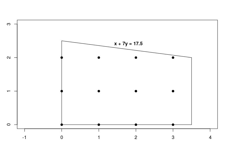
Tieni presente che questo problema è molto simile a quello dell'ottimizzazione lineare descritto nella sezione Risolvere un problema di pagina di destinazione, ma in questo caso le soluzioni devono essere numeri interi.
Passaggi di base per risolvere un problema MIP
Per risolvere un problema MIP, il tuo programma deve includere i seguenti passaggi:
- Importa il wrapper del risolutore lineare,
- dichiarare il risolutore MIP,
- a definire le variabili,
- definiscono i vincoli,
- definiscono l'obiettivo,
- chiama il risolutore MIP
- visualizza la soluzione
Soluzione che utilizza MPSolver
La seguente sezione presenta un programma che risolve il problema utilizzando il wrapper MPSolver e un risolutore MIP.
Il risolutore MIP predefinito OR-Tools è SCIP.
Importa il wrapper del risolutore lineare
Importa (o includi) il wrapper per il risolutore lineare OR-Tools, un'interfaccia per i risolutori MIP e lineari, come mostrato di seguito.
Python
from ortools.linear_solver import pywraplp
C++
#include <memory>

#include "ortools/linear_solver/linear_solver.h"
Java
import com.google.ortools.Loader;
import com.google.ortools.linearsolver.MPConstraint;
import com.google.ortools.linearsolver.MPObjective;
import com.google.ortools.linearsolver.MPSolver;
import com.google.ortools.linearsolver.MPVariable;
C#
using System;
using Google.OrTools.LinearSolver;
Dichiara il risolutore MIP
Il codice seguente dichiara il risolutore MIP per il problema. Questo esempio utilizza il risolutore di terze parti SCIP.
Python
# Create the mip solver with the SCIP backend.
solver = pywraplp.Solver.CreateSolver("SAT")
if not solver:
    return
C++
// Create the mip solver with the SCIP backend.
std::unique_ptr<MPSolver> solver(MPSolver::CreateSolver("SCIP"));
if (!solver) {
  LOG(WARNING) << "SCIP solver unavailable.";
  return;
}
Java
// Create the linear solver with the SCIP backend.
MPSolver solver = MPSolver.createSolver("SCIP");
if (solver == null) {
  System.out.println("Could not create solver SCIP");
  return;
}
C#
// Create the linear solver with the SCIP backend.
Solver solver = Solver.CreateSolver("SCIP");
if (solver is null)
{
    return;
}
Definisci le variabili
Il codice seguente definisce le variabili del problema.
Python
infinity = solver.infinity()
# x and y are integer non-negative variables.
x = solver.IntVar(0.0, infinity, "x")
y = solver.IntVar(0.0, infinity, "y")

print("Number of variables =", solver.NumVariables())
C++
const double infinity = solver->infinity();
// x and y are integer non-negative variables.
MPVariable* const x = solver->MakeIntVar(0.0, infinity, "x");
MPVariable* const y = solver->MakeIntVar(0.0, infinity, "y");

LOG(INFO) << "Number of variables = " << solver->NumVariables();
Java
double infinity = java.lang.Double.POSITIVE_INFINITY;
// x and y are integer non-negative variables.
MPVariable x = solver.makeIntVar(0.0, infinity, "x");
MPVariable y = solver.makeIntVar(0.0, infinity, "y");

System.out.println("Number of variables = " + solver.numVariables());
C#
// x and y are integer non-negative variables.
Variable x = solver.MakeIntVar(0.0, double.PositiveInfinity, "x");
Variable y = solver.MakeIntVar(0.0, double.PositiveInfinity, "y");

Console.WriteLine("Number of variables = " + solver.NumVariables());
Il programma utilizza il metodo MakeIntVar (o una variante, a seconda del linguaggio di programmazione) per creare variabili x e y che assumono valori interi non negativi.
Definisci i vincoli
Il codice seguente definisce i vincoli per il problema.
Python
# x + 7 * y <= 17.5.
solver.Add(x + 7 * y <= 17.5)

# x <= 3.5.
solver.Add(x <= 3.5)

print("Number of constraints =", solver.NumConstraints())
C++
// x + 7 * y <= 17.5.
MPConstraint* const c0 = solver->MakeRowConstraint(-infinity, 17.5, "c0");
c0->SetCoefficient(x, 1);
c0->SetCoefficient(y, 7);

// x <= 3.5.
MPConstraint* const c1 = solver->MakeRowConstraint(-infinity, 3.5, "c1");
c1->SetCoefficient(x, 1);
c1->SetCoefficient(y, 0);

LOG(INFO) << "Number of constraints = " << solver->NumConstraints();
Java
// x + 7 * y <= 17.5.
MPConstraint c0 = solver.makeConstraint(-infinity, 17.5, "c0");
c0.setCoefficient(x, 1);
c0.setCoefficient(y, 7);

// x <= 3.5.
MPConstraint c1 = solver.makeConstraint(-infinity, 3.5, "c1");
c1.setCoefficient(x, 1);
c1.setCoefficient(y, 0);

System.out.println("Number of constraints = " + solver.numConstraints());
C#
// x + 7 * y <= 17.5.
solver.Add(x + 7 * y <= 17.5);

// x <= 3.5.
solver.Add(x <= 3.5);

Console.WriteLine("Number of constraints = " + solver.NumConstraints());
Definire l'obiettivo
Il codice seguente definisce objective function per il problema.
Python
# Maximize x + 10 * y.
solver.Maximize(x + 10 * y)
C++
// Maximize x + 10 * y.
MPObjective* const objective = solver->MutableObjective();
objective->SetCoefficient(x, 1);
objective->SetCoefficient(y, 10);
objective->SetMaximization();
Java
// Maximize x + 10 * y.
MPObjective objective = solver.objective();
objective.setCoefficient(x, 1);
objective.setCoefficient(y, 10);
objective.setMaximization();
C#
// Maximize x + 10 * y.
solver.Maximize(x + 10 * y);
Chiama il risolutore
Il codice seguente chiama il risolutore.
Python
print(f"Solving with {solver.SolverVersion()}")
status = solver.Solve()
C++
const MPSolver::ResultStatus result_status = solver->Solve();
// Check that the problem has an optimal solution.
if (result_status != MPSolver::OPTIMAL) {
  LOG(FATAL) << "The problem does not have an optimal solution!";
}
Java
final MPSolver.ResultStatus resultStatus = solver.solve();
C#
Solver.ResultStatus resultStatus = solver.Solve();
Visualizza la soluzione
Il codice seguente mostra la soluzione.
Python
if status == pywraplp.Solver.OPTIMAL:
    print("Solution:")
    print("Objective value =", solver.Objective().Value())
    print("x =", x.solution_value())
    print("y =", y.solution_value())
else:
    print("The problem does not have an optimal solution.")
C++
LOG(INFO) << "Solution:";
LOG(INFO) << "Objective value = " << objective->Value();
LOG(INFO) << "x = " << x->solution_value();
LOG(INFO) << "y = " << y->solution_value();
Java
if (resultStatus == MPSolver.ResultStatus.OPTIMAL) {
  System.out.println("Solution:");
  System.out.println("Objective value = " + objective.value());
  System.out.println("x = " + x.solutionValue());
  System.out.println("y = " + y.solutionValue());
} else {
  System.err.println("The problem does not have an optimal solution!");
}
C#
// Check that the problem has an optimal solution.
if (resultStatus != Solver.ResultStatus.OPTIMAL)
{
    Console.WriteLine("The problem does not have an optimal solution!");
    return;
}
Console.WriteLine("Solution:");
Console.WriteLine("Objective value = " + solver.Objective().Value());
Console.WriteLine("x = " + x.SolutionValue());
Console.WriteLine("y = " + y.SolutionValue());
Di seguito è riportata la soluzione al problema.
Number of variables = 2
Number of constraints = 2
Solution:
Objective value = 23
x = 3
y = 2
Il valore ottimale della funzione obiettivo è 23, che si verifica nel punto x = 3, y = 2.
Completa i programmi
Ecco i programmi completi.
Python
from ortools.linear_solver import pywraplp


def main():
    # Create the mip solver with the SCIP backend.
    solver = pywraplp.Solver.CreateSolver("SAT")
    if not solver:
        return

    infinity = solver.infinity()
    # x and y are integer non-negative variables.
    x = solver.IntVar(0.0, infinity, "x")
    y = solver.IntVar(0.0, infinity, "y")

    print("Number of variables =", solver.NumVariables())

    # x + 7 * y <= 17.5.
    solver.Add(x + 7 * y <= 17.5)

    # x <= 3.5.
    solver.Add(x <= 3.5)

    print("Number of constraints =", solver.NumConstraints())

    # Maximize x + 10 * y.
    solver.Maximize(x + 10 * y)

    print(f"Solving with {solver.SolverVersion()}")
    status = solver.Solve()

    if status == pywraplp.Solver.OPTIMAL:
        print("Solution:")
        print("Objective value =", solver.Objective().Value())
        print("x =", x.solution_value())
        print("y =", y.solution_value())
    else:
        print("The problem does not have an optimal solution.")

    print("\nAdvanced usage:")
    print(f"Problem solved in {solver.wall_time():d} milliseconds")
    print(f"Problem solved in {solver.iterations():d} iterations")
    print(f"Problem solved in {solver.nodes():d} branch-and-bound nodes")


if __name__ == "__main__":
    main()
C++
#include <memory>

#include "ortools/linear_solver/linear_solver.h"

namespace operations_research {
void SimpleMipProgram() {
  // Create the mip solver with the SCIP backend.
  std::unique_ptr<MPSolver> solver(MPSolver::CreateSolver("SCIP"));
  if (!solver) {
    LOG(WARNING) << "SCIP solver unavailable.";
    return;
  }

  const double infinity = solver->infinity();
  // x and y are integer non-negative variables.
  MPVariable* const x = solver->MakeIntVar(0.0, infinity, "x");
  MPVariable* const y = solver->MakeIntVar(0.0, infinity, "y");

  LOG(INFO) << "Number of variables = " << solver->NumVariables();

  // x + 7 * y <= 17.5.
  MPConstraint* const c0 = solver->MakeRowConstraint(-infinity, 17.5, "c0");
  c0->SetCoefficient(x, 1);
  c0->SetCoefficient(y, 7);

  // x <= 3.5.
  MPConstraint* const c1 = solver->MakeRowConstraint(-infinity, 3.5, "c1");
  c1->SetCoefficient(x, 1);
  c1->SetCoefficient(y, 0);

  LOG(INFO) << "Number of constraints = " << solver->NumConstraints();

  // Maximize x + 10 * y.
  MPObjective* const objective = solver->MutableObjective();
  objective->SetCoefficient(x, 1);
  objective->SetCoefficient(y, 10);
  objective->SetMaximization();

  const MPSolver::ResultStatus result_status = solver->Solve();
  // Check that the problem has an optimal solution.
  if (result_status != MPSolver::OPTIMAL) {
    LOG(FATAL) << "The problem does not have an optimal solution!";
  }

  LOG(INFO) << "Solution:";
  LOG(INFO) << "Objective value = " << objective->Value();
  LOG(INFO) << "x = " << x->solution_value();
  LOG(INFO) << "y = " << y->solution_value();

  LOG(INFO) << "\nAdvanced usage:";
  LOG(INFO) << "Problem solved in " << solver->wall_time() << " milliseconds";
  LOG(INFO) << "Problem solved in " << solver->iterations() << " iterations";
  LOG(INFO) << "Problem solved in " << solver->nodes()
            << " branch-and-bound nodes";
}
}  // namespace operations_research

int main(int argc, char** argv) {
  operations_research::SimpleMipProgram();
  return EXIT_SUCCESS;
}
Java
package com.google.ortools.linearsolver.samples;
import com.google.ortools.Loader;
import com.google.ortools.linearsolver.MPConstraint;
import com.google.ortools.linearsolver.MPObjective;
import com.google.ortools.linearsolver.MPSolver;
import com.google.ortools.linearsolver.MPVariable;

/** Minimal Mixed Integer Programming example to showcase calling the solver. */
public final class SimpleMipProgram {
  public static void main(String[] args) {
    Loader.loadNativeLibraries();
    // Create the linear solver with the SCIP backend.
    MPSolver solver = MPSolver.createSolver("SCIP");
    if (solver == null) {
      System.out.println("Could not create solver SCIP");
      return;
    }

    double infinity = java.lang.Double.POSITIVE_INFINITY;
    // x and y are integer non-negative variables.
    MPVariable x = solver.makeIntVar(0.0, infinity, "x");
    MPVariable y = solver.makeIntVar(0.0, infinity, "y");

    System.out.println("Number of variables = " + solver.numVariables());

    // x + 7 * y <= 17.5.
    MPConstraint c0 = solver.makeConstraint(-infinity, 17.5, "c0");
    c0.setCoefficient(x, 1);
    c0.setCoefficient(y, 7);

    // x <= 3.5.
    MPConstraint c1 = solver.makeConstraint(-infinity, 3.5, "c1");
    c1.setCoefficient(x, 1);
    c1.setCoefficient(y, 0);

    System.out.println("Number of constraints = " + solver.numConstraints());

    // Maximize x + 10 * y.
    MPObjective objective = solver.objective();
    objective.setCoefficient(x, 1);
    objective.setCoefficient(y, 10);
    objective.setMaximization();

    final MPSolver.ResultStatus resultStatus = solver.solve();

    if (resultStatus == MPSolver.ResultStatus.OPTIMAL) {
      System.out.println("Solution:");
      System.out.println("Objective value = " + objective.value());
      System.out.println("x = " + x.solutionValue());
      System.out.println("y = " + y.solutionValue());
    } else {
      System.err.println("The problem does not have an optimal solution!");
    }

    System.out.println("\nAdvanced usage:");
    System.out.println("Problem solved in " + solver.wallTime() + " milliseconds");
    System.out.println("Problem solved in " + solver.iterations() + " iterations");
    System.out.println("Problem solved in " + solver.nodes() + " branch-and-bound nodes");
  }

  private SimpleMipProgram() {}
}
C#
using System;
using Google.OrTools.LinearSolver;

public class SimpleMipProgram
{
    static void Main()
    {
        // Create the linear solver with the SCIP backend.
        Solver solver = Solver.CreateSolver("SCIP");
        if (solver is null)
        {
            return;
        }

        // x and y are integer non-negative variables.
        Variable x = solver.MakeIntVar(0.0, double.PositiveInfinity, "x");
        Variable y = solver.MakeIntVar(0.0, double.PositiveInfinity, "y");

        Console.WriteLine("Number of variables = " + solver.NumVariables());

        // x + 7 * y <= 17.5.
        solver.Add(x + 7 * y <= 17.5);

        // x <= 3.5.
        solver.Add(x <= 3.5);

        Console.WriteLine("Number of constraints = " + solver.NumConstraints());

        // Maximize x + 10 * y.
        solver.Maximize(x + 10 * y);

        Solver.ResultStatus resultStatus = solver.Solve();

        // Check that the problem has an optimal solution.
        if (resultStatus != Solver.ResultStatus.OPTIMAL)
        {
            Console.WriteLine("The problem does not have an optimal solution!");
            return;
        }
        Console.WriteLine("Solution:");
        Console.WriteLine("Objective value = " + solver.Objective().Value());
        Console.WriteLine("x = " + x.SolutionValue());
        Console.WriteLine("y = " + y.SolutionValue());

        Console.WriteLine("\nAdvanced usage:");
        Console.WriteLine("Problem solved in " + solver.WallTime() + " milliseconds");
        Console.WriteLine("Problem solved in " + solver.Iterations() + " iterations");
        Console.WriteLine("Problem solved in " + solver.Nodes() + " branch-and-bound nodes");
    }
}
Confronto tra l'ottimizzazione di numeri interi e lineari
Confrontiamo la soluzione con il problema di ottimizzazione dei numeri interi, mostrato sopra, con il corrispondente problema di ottimizzazione lineare, in cui i vincoli con numeri interi vengono rimossi. Potresti immaginare che la soluzione al problema con il numero intero sia il punto intero nella regione fattibile più vicina alla soluzione lineare, ovvero il punto x = 0, y = 2. Ma, come vedremo in seguito,
non è così.
Puoi modificare facilmente il programma nella sezione precedente per risolvere il problema lineare apportando le seguenti modifiche:
- Sostituisci il risolutore MIP
con il risolutore LP
Python
# Create the mip solver with the SCIP backend.
solver = pywraplp.Solver.CreateSolver("SAT")
if not solver:
    return
C++
// Create the mip solver with the SCIP backend.
std::unique_ptr<MPSolver> solver(MPSolver::CreateSolver("SCIP"));
if (!solver) {
  LOG(WARNING) << "SCIP solver unavailable.";
  return;
}
Java
// Create the linear solver with the SCIP backend.
MPSolver solver = MPSolver.createSolver("SCIP");
if (solver == null) {
  System.out.println("Could not create solver SCIP");
  return;
}
C#
// Create the linear solver with the SCIP backend. Solver solver = Solver.CreateSolver("SCIP"); if (solver is null) { return; }Python
# Create the linear solver with the GLOP backend.
solver = pywraplp.Solver.CreateSolver("GLOP")
if not solver:
    return
C++
// Create the linear solver with the GLOP backend.
std::unique_ptr<MPSolver> solver(MPSolver::CreateSolver("GLOP"));
Java
// Create the linear solver with the GLOP backend.
MPSolver solver = MPSolver.createSolver("GLOP");
if (solver == null) {
  System.out.println("Could not create solver SCIP");
  return;
}
C#
// Create the linear solver with the GLOP backend. Solver solver = Solver.CreateSolver("GLOP"); if (solver is null) { return; } - Sostituisci le variabili con numeri interi
con variabili continue
Python
infinity = solver.infinity()
# x and y are integer non-negative variables.
x = solver.IntVar(0.0, infinity, "x")
y = solver.IntVar(0.0, infinity, "y")

print("Number of variables =", solver.NumVariables())
C++
const double infinity = solver->infinity();
// x and y are integer non-negative variables.
MPVariable* const x = solver->MakeIntVar(0.0, infinity, "x");
MPVariable* const y = solver->MakeIntVar(0.0, infinity, "y");

LOG(INFO) << "Number of variables = " << solver->NumVariables();
Java
double infinity = java.lang.Double.POSITIVE_INFINITY;
// x and y are integer non-negative variables.
MPVariable x = solver.makeIntVar(0.0, infinity, "x");
MPVariable y = solver.makeIntVar(0.0, infinity, "y");

System.out.println("Number of variables = " + solver.numVariables());
C#
// x and y are integer non-negative variables. Variable x = solver.MakeIntVar(0.0, double.PositiveInfinity, "x"); Variable y = solver.MakeIntVar(0.0, double.PositiveInfinity, "y"); Console.WriteLine("Number of variables = " + solver.NumVariables());Python
infinity = solver.infinity()
# Create the variables x and y.
x = solver.NumVar(0.0, infinity, "x")
y = solver.NumVar(0.0, infinity, "y")

print("Number of variables =", solver.NumVariables())
C++
const double infinity = solver->infinity();
// Create the variables x and y.
MPVariable* const x = solver->MakeNumVar(0.0, infinity, "x");
MPVariable* const y = solver->MakeNumVar(0.0, infinity, "y");

LOG(INFO) << "Number of variables = " << solver->NumVariables();
Java
double infinity = java.lang.Double.POSITIVE_INFINITY;
// Create the variables x and y.
MPVariable x = solver.makeNumVar(0.0, infinity, "x");
MPVariable y = solver.makeNumVar(0.0, infinity, "y");

System.out.println("Number of variables = " + solver.numVariables());
C#
// Create the variables x and y.
Variable x = solver.MakeNumVar(0.0, double.PositiveInfinity, "x");
Variable y = solver.MakeNumVar(0.0, double.PositiveInfinity, "y");

Console.WriteLine("Number of variables = " + solver.NumVariables());
Dopo aver apportato queste modifiche ed eseguito di nuovo il programma, ottieni il seguente output:
Number of variables = 2
Number of constraints = 2
Objective value = 25.000000
x = 0.000000
y = 2.500000
La soluzione al problema lineare si verifica nel punto x = 0, y = 2.5, dove
la funzione obiettivo è uguale a 25. Ecco un grafico che mostra le soluzioni
ai problemi lineari e interi.
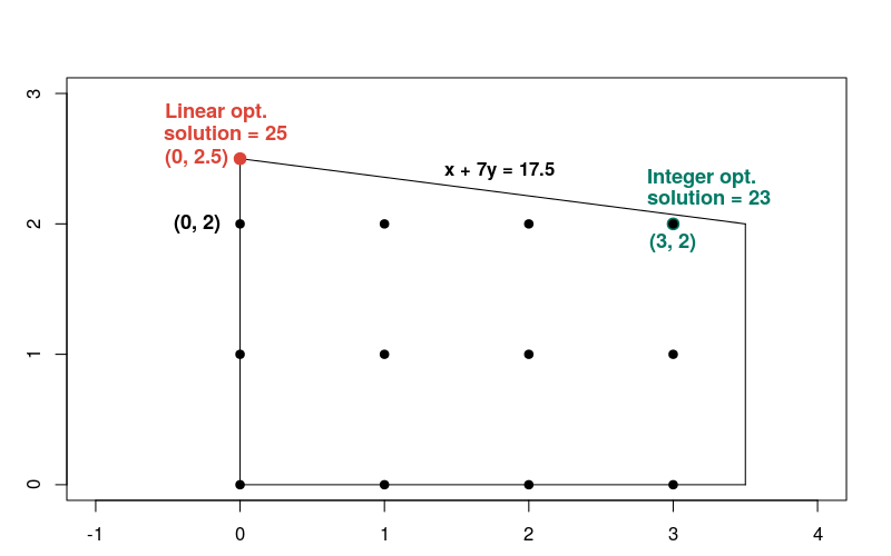
Nota che la soluzione intera non è vicina alla soluzione lineare, rispetto alla maggior parte degli altri punti interi nella regione fattibile. In generale, le soluzioni a un problema di ottimizzazione lineare e i corrispondenti problemi di ottimizzazione con numeri interi possono essere distanziati. Per questo motivo, i due tipi di problemi richiedono metodi diversi per risolverlo.