Page Summary
-
Imbalanced datasets occur when one label (majority class) is significantly more frequent than another (minority class), potentially hindering model training on the minority class.
-
Downsampling the majority class and upweighting it can improve model performance by balancing class representation and reducing prediction bias.
-
Experimenting with rebalancing ratios is crucial for optimal performance, ensuring batches contain enough minority class examples for effective training.
-
Upweighting the minority class is simpler but may increase prediction bias compared to downsampling and upweighting the majority class.
-
Downsampling offers benefits like faster convergence and less disk space usage but requires manual effort, especially for large datasets.
This section explores the following three questions:
- What's the difference between class-balanced datasets and class-imbalanced datasets?
- Why is training an imbalanced dataset difficult?
- How can you overcome the problems of training imbalanced datasets?
Class-balanced datasets versus class-imbalanced datasets
Consider a dataset containing a categorical label whose value is either the positive class or the negative class. In a class-balanced dataset, the number of positive classes and negative classes is about equal. For example, a dataset containing 235 positive classes and 247 negative classes is a balanced dataset.
In a class-imbalanced dataset, one label is considerably more common than the other. In the real world, class-imbalanced datasets are far more common than class-balanced datasets. For example, in a dataset of credit card transactions, fraudulent purchases might make up less than 0.1% of the examples. Similarly, in a medical diagnosis dataset, the number of patients with a rare virus might be less than 0.01% of the total examples. In a class-imbalanced dataset:
- The more common label is called the majority class.
- The less common label is called the minority class.
The difficulty of training severely class-imbalanced datasets
Training aims to create a model that successfully distinguishes the positive class from the negative class. To do so, batches need a sufficient number of both positive classes and negative classes. That's not a problem when training on a mildly class-imbalanced dataset since even small batches typically contain sufficient examples of both the positive class and the negative class. However, a severely class-imbalanced dataset might not contain enough minority class examples for proper training.
For example, consider the class-imbalanced dataset illustrated in Figure 6 in which:
- 200 labels are in the majority class.
- 2 labels are in the minority class.
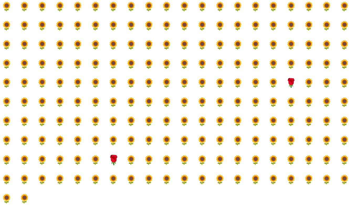
If the batch size is 20, most batches won't contain any examples of the minority class. If the batch size is 100, each batch will contain an average of only one minority class example, which is insufficient for proper training. Even a much larger batch size will still yield such an imbalanced proportion that the model might not train properly.
Training a class-imbalanced dataset
During training, a model should learn two things:
- What each class looks like; that is, what feature values correspond to what class?
- How common each class is; that is, what is the relative distribution of the classes?
Standard training conflates these two goals. In contrast, the following two-step technique called downsampling and upweighting the majority class separates these two goals, enabling the model to achieve both goals.
Step 1: Downsample the majority class
Downsampling means training on a disproportionately low percentage of majority class examples. That is, you artificially force a class-imbalanced dataset to become somewhat more balanced by omitting many of the majority class examples from training. Downsampling greatly increases the probability that each batch contains enough examples of the minority class to train the model properly and efficiently.
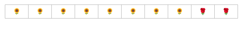
For example, the class-imbalanced dataset shown in Figure 6 consists of 99% majority class and 1% minority class examples. Downsampling the majority class by a factor of 25 artificially creates a more balanced training set (80% majority class to 20% minority class) suggested in Figure 7:
Step 2: Upweight the downsampled class
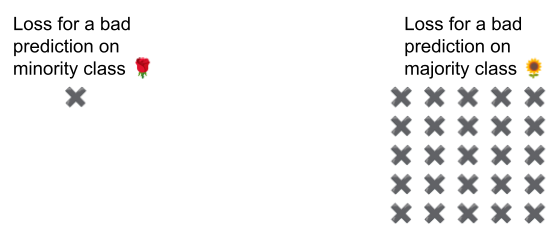
Downsampling introduces a prediction bias by showing the model an artificial world where the classes are more balanced than in the real world. To correct this bias, you must "upweight" the majority classes by the factor to which you downsampled. Upweighting means treating the loss on a majority class example more harshly than the loss on a minority class example.
For example, we downsampled the majority class by a factor of 25, so we must upweight the majority class by a factor of 25. That is, when the model mistakenly predicts the majority class, treat the loss as if it were 25 errors (multiply the regular loss by 25).
How much should you downsample and upweight to rebalance your dataset? To determine the answer, you should experiment with different downsampling and upweighting factors just as you would experiment with other hyperparameters.
Benefits of this technique
Downsampling and upweighting the majority class brings the following benefits:
- Better model: The resultant model "knows" both of the following:
- The connection between features and labels
- The true distribution of the classes
- Faster convergence: During training, the model sees the minority class more often, which helps the model converge faster.