Non-Parametric Trend Analysis

Author(s): n-clinton

Trend analysis is finding places where something of interest is increasing or decreasing and by how much. More specifically, this tutorial demonstrates detecting monotonic trends in imagery using the non-parametric Mann-Kendall test for the presence of an increasing or decreasing trend and Sen's slope to quantify the magnitude of the trend (if one exists). The tutorial also shows estimating the variance of the Mann-Kendall test statistic, a Z-statistic for the test of presence of any trend, and a P-value of the statistic (assuming a normal distribution).

Important: the methods presented here are suitable for assessing monotonic trends (i.e. data without seasonality) in discrete data (i.e. not floating point). Additionally, if you apply the methods in this tutorial to new data (i.e. region, time frame, source) you may need to adjust the min and max visualization parameters to suit the particular results.

Time series data

We will use a time series of MODIS Enhanced Vegetation Index (EVI) from the MOD13A1 dataset. Each pixel of this image collection contains a time series and we will compute the stats in each pixel. Assume that filtering the collection to one season is sufficient to obtain time series with monotonic trends. To check the validity of that assumption for your area of interest, add the collection to the map and using the inspector, click some points and view the series chart presented in the console. Adjust the filter as necessary.

var mod13 = ee.ImageCollection('MODIS/006/MOD13A1');
var coll = mod13.select('EVI')
    .filter(ee.Filter.calendarRange(8, 9, 'month'));
Map.setCenter(-121.6, 37.3, 10);
Map.addLayer(coll, {min: -500, max: 5000, palette: ['white', 'green']}, 'coll');

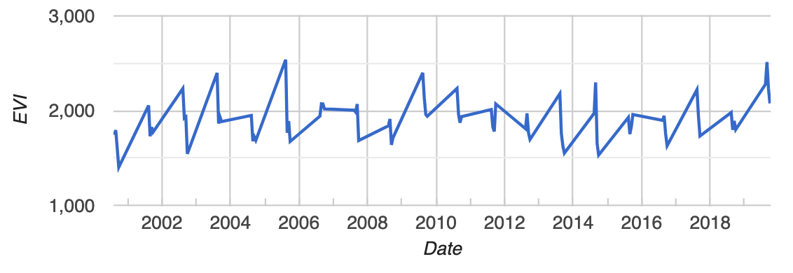
An example EVI time series (one pixel) from this collection is shown below. Is there a trend in this pixel? More importantly, is a there a statistically significant trend in this pixel? Read on to find out!

EVI time series in a single pixel

Join the time series to itself

The non-parametric stats of interest are computed by examining every possible ordered pair of unique values in the time series. If there are n time points in the series, we need to examine the n(n-1)/2 pairs (i, j), i<j, where i and j are arbitrary time indices. (Here we use (i, j) to signify the pair of EVI images indexed by i and j). To do that, join the collection to itself with a temporal filter. The temporal filter will pass all the chronologically later images. In the joined collection, each image will store all the images that come after it in an after property.

var afterFilter = ee.Filter.lessThan({
  leftField: 'system:time_start',
  rightField: 'system:time_start'
});

var joined = ee.ImageCollection(ee.Join.saveAll('after').apply({
  primary: coll,
  secondary: coll,
  condition: afterFilter
}));

Mann-Kendall trend test

The Mann-Kendall trend is defined as the sum of the signs of all the pairs. The sign is 1 if EVI at time j is more than EVI at time i, -1 if the opposite is true and zero otherwise (if they're equal). Compute this by iterating over the collection and computing sign(i, j) for each image i in the collection and each image j in the after images.

var sign = function(i, j) { // i and j are images
  return ee.Image(j).neq(i) // Zero case
      .multiply(ee.Image(j).subtract(i).clamp(-1, 1)).int();
};

var kendall = ee.ImageCollection(joined.map(function(current) {
  var afterCollection = ee.ImageCollection.fromImages(current.get('after'));
  return afterCollection.map(function(image) {
    // The unmask is to prevent accumulation of masked pixels that
    // result from the undefined case of when either current or image
    // is masked.  It won't affect the sum, since it's unmasked to zero.
    return ee.Image(sign(current, image)).unmask(0);
  });
  // Set parallelScale to avoid User memory limit exceeded.
}).flatten()).reduce('sum', 2);

var palette = ['red', 'white', 'green'];
// Set min and max stretch visualization parameters as necessary.
Map.addLayer(kendall, {palette: palette, min: -2800, max: 2800}, 'kendall');

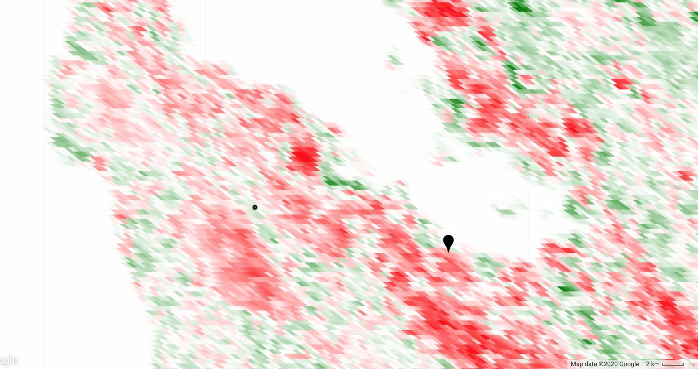
Zoom to your area of interest and define a roughly symmetric color stretch using the map layers styling dialog (i.e. the mean of min and max should be approximately zero). The red pixels are decreasing trend and the green pixels are increasing trend. This is illustrated in the following image of the Mann-Kendall statistic for an area of California, USA. The map pin is at the approximate location of the Googleplex. The dot is the location of the point from which the time series shown above was extracted. We'd like to identify which pixels in this map have significant trend.

Mann Kendall Statistic Map

You may also be interested in knowing the magnitude of the trend, or the slope of the trend over time in the present context. A non-parametric way of assessing that is with Sen's slope.

Sen's slope

Sen's slope is computed in a similar way to the Mann-Kendall statistic. However, instead of adding all the signs of the pairs, the slope is computed for all the pairs. Sen's slope is the median slope from all those pairs. In the following, slope is computed over days to avoid numerically tiny slopes (which might result from using epoch time instead).

var slope = function(i, j) { // i and j are images
  return ee.Image(j).subtract(i)
      .divide(ee.Image(j).date().difference(ee.Image(i).date(), 'days'))
      .rename('slope')
      .float();
};

var slopes = ee.ImageCollection(joined.map(function(current) {
  var afterCollection = ee.ImageCollection.fromImages(current.get('after'));
  return afterCollection.map(function(image) {
      return ee.Image(slope(current, image));
  });
}).flatten());

var sensSlope = slopes.reduce(ee.Reducer.median(), 2); // Set parallelScale.
Map.addLayer(sensSlope, {palette: palette, min: -1, max: 1}, 'sensSlope');

To get Sen's intercept (if you need it), compute all intercepts and take the median.

var epochDate = ee.Date('1970-01-01');
var sensIntercept = coll.map(function(image) {
  var epochDays = image.date().difference(epochDate, 'days').float();
  return image.subtract(sensSlope.multiply(epochDays)).float();
}).reduce(ee.Reducer.median(), 2);
Map.addLayer(sensIntercept, {min: -6600, max: 20600}, 'sensIntercept');

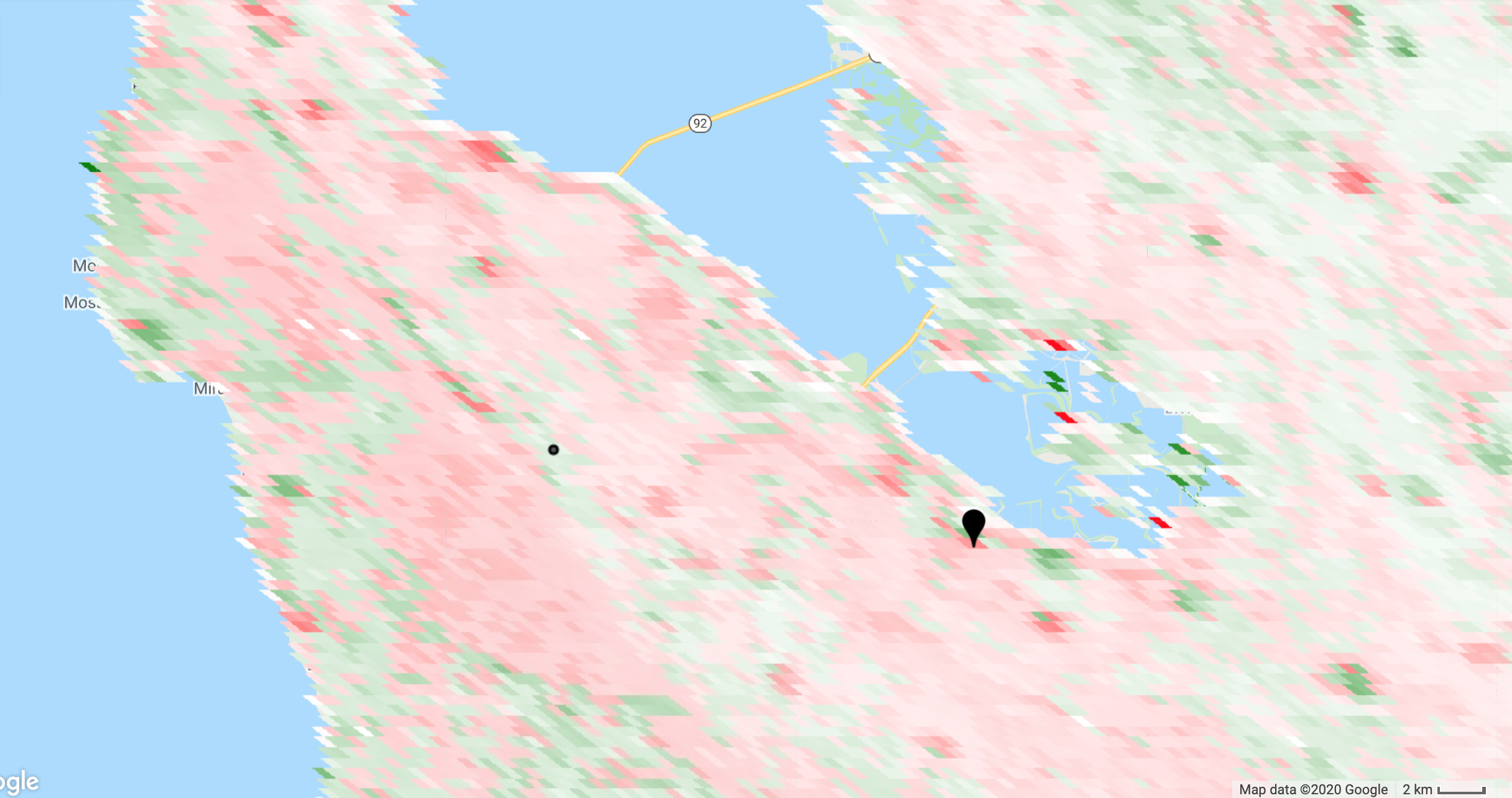
A map of Sen's slope is shown below. Note that the pattern is similar to the Mann-Kendall statistic, but not identical. Also, there is still the question of which pixels have significant trend, a question that will be answered shortly.

Sens Slope Map

The previous examples are only to demonstrate the computation. If you need Sen's slope and/or intercept, you can also use the Sen's slope reducer which is likely to be easier (less code) and more efficient, but computes the intercept as the y-value of the line that passes through the medians.

Variance of the Mann-Kendall statistic

Computing the variance of the Mann-Kendall statistic is complicated by the possible presence of ties in the data (i.e. sign(i, j) equals zero). Counting those ties can get a little dicey, requiring an array-based forward differencing. Note that you can comment .subtract(groupFactorSum) in the computation of kendallVariance if you don't care about ties and want to disregard that correction.

// Values that are in a group (ties).  Set all else to zero.
var groups = coll.map(function(i) {
  var matches = coll.map(function(j) {
    return i.eq(j); // i and j are images.
  }).sum();
  return i.multiply(matches.gt(1));
});

// Compute tie group sizes in a sequence.  The first group is discarded.
var group = function(array) {
  var length = array.arrayLength(0);
  // Array of indices.  These are 1-indexed.
  var indices = ee.Image([1])
      .arrayRepeat(0, length)
      .arrayAccum(0, ee.Reducer.sum())
      .toArray(1);
  var sorted = array.arraySort();
  var left = sorted.arraySlice(0, 1);
  var right = sorted.arraySlice(0, 0, -1);
  // Indices of the end of runs.
  var mask = left.neq(right)
  // Always keep the last index, the end of the sequence.
      .arrayCat(ee.Image(ee.Array([[1]])), 0);
  var runIndices = indices.arrayMask(mask);
  // Subtract the indices to get run lengths.
  var groupSizes = runIndices.arraySlice(0, 1)
      .subtract(runIndices.arraySlice(0, 0, -1));
  return groupSizes;
};

// See equation 2.6 in Sen (1968).
var factors = function(image) {
  return image.expression('b() * (b() - 1) * (b() * 2 + 5)');
};

var groupSizes = group(groups.toArray());
var groupFactors = factors(groupSizes);
var groupFactorSum = groupFactors.arrayReduce('sum', [0])
      .arrayGet([0, 0]);

var count = joined.count();

var kendallVariance = factors(count)
    .subtract(groupFactorSum)
    .divide(18)
    .float();
Map.addLayer(kendallVariance, {min: 1700, max: 85000}, 'kendallVariance');

Significance testing

The Mann-Kendall statistic is asymptotically normal for suitably large samples. Assume our samples are suitably large and uncorrelated. Under these assumptions, the true mean of the Mann-Kendall statistic is zero and the variance is as computed above. To compute a standard normal statistic (z), divide the statistic by its standard deviation. The P-value of the z-statistic (probability of observing such an extreme value) is 1 - P(|z| < Z). For a two-sided test of whether any trend exists (positive or negative) at the 95% confidence level, compare the P-value to 0.975. (Alternatively, compare the z-statistic to Z*, where Z* is the inverse distribution function of 0.975).

The standard normal distribution function can be computed in Earth Engine from the error function, erf(). Both the distribution function and its inverse are shown below for reference. Here we use the distribution function to get 1 - P(|z| < Z) and compare it to 0.975.

// Compute Z-statistics.
var zero = kendall.multiply(kendall.eq(0));
var pos = kendall.multiply(kendall.gt(0)).subtract(1);
var neg = kendall.multiply(kendall.lt(0)).add(1);

var z = zero
    .add(pos.divide(kendallVariance.sqrt()))
    .add(neg.divide(kendallVariance.sqrt()));
Map.addLayer(z, {min: -2, max: 2}, 'z');

// https://en.wikipedia.org/wiki/Error_function#Cumulative_distribution_function
function eeCdf(z) {
  return ee.Image(0.5)
      .multiply(ee.Image(1).add(ee.Image(z).divide(ee.Image(2).sqrt()).erf()));
}

function invCdf(p) {
  return ee.Image(2).sqrt()
      .multiply(ee.Image(p).multiply(2).subtract(1).erfInv());
}

// Compute P-values.
var p = ee.Image(1).subtract(eeCdf(z.abs()));
Map.addLayer(p, {min: 0, max: 1}, 'p');

// Pixels that can have the null hypothesis (there is no trend) rejected.
// Specifically, if the true trend is zero, there would be less than 5%
// chance of randomly obtaining the observed result (that there is a trend).
Map.addLayer(p.lte(0.025), {min: 0, max: 1}, 'significant trends');

The following shows a map of the "significant" pixels (in white), or the pixels that pass the p.lte(0.025) test. If our assumptions are correct and you are satisfied with the computation, you may wish to treat these pixels differently, by using p.lte(0.025) as a mask. Note that the pixel with the time series shown above (red in the map below) does NOT have a significant trend.

Statistically Significant Pixels

Some call this process significance testing. Pixels that are "significant" satisfy the condition that p.lte(0.025) and are assumed to have a real trend. Other pixels are assumed to not have a trend and are removed from further analysis. Some consider this process cultish (Ziliak and McCloskey 2009). You decide!

References

- Thiel. 1950. A rank-invariant method of linear and polynomial regression analysis.
- Sen. 1968. Estimates of the Regression Coefficient Based on Kendall's Tau
- Morell and Fried 2009. On Nonparametric Tests for Trend Detection in Seasonal Time Series
- Pohlert 2020. Non-Parametric Trend Tests and Change-Point Detection