
Meridian's default ROI priors are moderately informative. One of the most helpful ways to improve the estimates of your Meridian model is to calibrate ROI priors with incrementality experiments. Incrementality testing establishes experimental ground truth to calibrate Meridian estimates, ensuring your ROI metrics reflect causal impact.
Because running experiments across all media channels is logistically complex and expensive, Meridian helps identify channels where the model exhibits high uncertainty, potential bias, or unrealistic baseline estimates to prioritize for testing. It does this by outputting a top level channel calibration recommendation and score for each channel in your MMM.
You can use these recommendations and scores to identify these channels and evaluate which ones would benefit most from having their ROI prior calibrated by an incrementality experiment, such as those executed with Meridian GeoX. For more information on how to set up and run a Meridian GeoX experiment, see Meridian GeoX.
Run channel calibration recommendation
Meridian channel calibration recommendation and scores are accessible in the model health report, which can be generated by running:
from IPython import display
from meridian.analysis.review import reviewer
from meridian.model import model

mmm = model.Meridian(...)
health_summary = reviewer.ModelReviewer(mmm).run()

filename = 'health_card.html'
health_summary.output_model_health_card(filename=filename, filepath=meridian_root)
display.HTML(filename=f'{meridian_root}{filename}')
Understand how Meridian proposes channels for calibration
Meridian proposes channels for calibration by computing a composite calibration score and flagging channels whose scores fall below 67.5. The composite calibration score is a unified measure of how much a given channel would benefit from calibration. It unifies the implausible ROI, high-variance ROI, and potential bias metrics into a single scalar score.
This composite score lets you distinguish between similarly flagged channels to decide which channels to prioritize:
- Higher scores (approaching 100): Considered healthier, would benefit less from calibration.
- Lower scores (approaching 0): Considered less healthy and would benefit more from calibration.
The overall composite calibration score is defined as the weighted average of three component scores: the Implausible ROI score, the High Variance ROI score, and the Potential Bias score. These scores are based on four individual channel recommendation criteria.
Channel recommendation criteria
Meridian has four checks when proposing media and reach and frequency channels for calibration:
- Implausibly high ROI estimates.
- Implausibly low ROI estimates.
- High variance ROI estimates.
- High potential bias.
The implausibly high ROI, implausibly low ROI and high variance ROI criteria are spend-weighted to account for the tendency of low-spend channels to have higher variance, which can result in extreme point estimates and wide posterior distributions. Spend-weighting also prioritizes calibration for higher-spend channels due to their greater business importance.
The overall calibration recommendation is based on the composite calibration score. If any criteria are flagged, they are labelled as a driver of channel calibration recommendation. Each of the criteria are explained in this section.
Implausibly high ROI
Meridian checks if implausibly high ROI is a driver of calibration recommendation by calculating the spend-weighted ROI and comparing it to a defined upper threshold, \(T_{\text{high_roi}}\). Channel \(i\) is a driver if its spend-weighted mean ROI exceeds the threshold:
\[ \frac{\text{spend}_{i}}{\sum_{j}\text{spend}_{j}}\cdot ROI_{i} > T_{\text{high_roi}} \]
where \(\text{spend}_{i}\) and \(ROI_{i}\) are the spend and ROI of channel \(i\), respectively, and the sum in the denominator is taken over all paid media and reach and frequency channels.
By default, \(T_{\text{high_roi}}=20\).
Implausibly low ROI
Similarly, Meridian checks if implausibly low ROI is a driver of calibration recommendation by calculating the reciprocal-spend-weighted ROI and compare it to a defined lower threshold, \(T_{\text{low_roi}}\). Meridian uses reciprocal-spend weighting in this case because the inequality is a lower bound. Channel \(i\) is a driver if its reciprocal-spend-weighted mean ROI falls below the threshold:
\[ \left(\frac{\text{spend}_{i}}{\sum_{j}\text{spend}_{j}}\right)^{-1} \cdot ROI_{i} < T_{\text{low_roi}} \]
where \(\text{spend}_{i}\) and \(ROI_{i}\) are the spend and ROI of channel \(i\), respectively, and the sum in the denominator is taken over all paid media and reach and frequency channels.
By default, \(T_{\text{low_roi}}=0.5\).
High variance ROI
This criterion identifies channels where the model's estimate is highly uncertain. Meridian checks for high variance by comparing the width of the channel's posterior ROI credible interval to the width of the Meridian default ROI prior credible interval (which defaults to LogNormal(0.2, 0.9)). This check compares the spend-weighted, normalized 80th percentile credible interval posterior width against the 80th percentile credible interval width of the default Meridian prior (LogNormal(0.2, 0.9)). Channel \(i\) is flagged if this relative width exceeds a threshold \(T_{\text{high_variance}}\). Specifically, let:
- \(\text{CI}^{(u)}\) be the 80th percentile credible interval upper bound of channel \(i\)'s posterior ROI,
- \(\text{CI}^{(l)}\) be the 80th percentile credible interval lower bound of channel \(i\)'s posterior ROI,
- \(\tilde{x} \) be the median of channel \(i\)'s posterior ROI,
- \(\text{CI}_\text{default}^{(u)}=2.64\) be the 80th percentile credible interval upper bound of the Meridian default ROI prior,
- \(\text{CI}_\text{default}^{(l)}=0.11\) be the 80th percentile credible interval lower bound of the Meridian default ROI prior, and
- \(\tilde{x}_\text{default}=1.22\) be the median of the Meridian default ROI prior.
The high variance ROI check is then
\[ \left(\frac{\text{spend}_{i}}{\sum_{j}\text{spend}_{j}}\right)\left(\frac{( \text{CI}^{(u)} - \text{CI}^{(l)} ) / \tilde{ x}}{(\text{CI}_\text{default}^{(u)} - \text{CI}_\text{default}^{(l)}) /\tilde{x}_\text{default} }\right) > T_\text{high_variance} \]
where \(\text{spend}_{i}\) is the spend of channel \(i\) and the sum in the denominator is taken over all paid media and reach and frequency channels
By default, \(T_\text{high_variance}=1.0\).
Potential bias (channels missing confounders)
Meridian posterior ROI estimates may be biased if models are missing key confounder variables. For example, if a model is missing a confounder for a holiday period, it may incorrectly estimate that natural sales increases were caused by channels that happened to increase spend during that same time. Experiment-based calibration helps correct this bias by grounding the model's ROI estimates in actual causal data.
Meridian checks for potential bias by computing, for each paid media and reach and frequency channel, the maximum absolute correlation with any control variable across all geos, and comparing it to a threshold \(T_\text{bias}\).
For a given paid media or reach and frequency channel \(i\), let \(E_{g,t,i}\) be its execution level:
\[ E_{g,t,i} = \begin{cases} x^{[M]}_{g,t,i} & \text{for paid media channels} \\ r^{[RF]}_{g,t,i} \cdot f^{[RF]}_{g,t,i} & \text{for paid reach and frequency channels} \end{cases} \]
where \(x^{[M]}_{g,t,i}\) is the execution of paid media channel \(i\) in geo \(g\) at time \(t\) and \(r^{[RF]}_{g,t,i}\) and \(f^{[RF]}_{g,t,i}\) are the reach and frequency of reach and frequency channel \(i\) in geo \(g\) at time \(t\), respectively.
The check flags channel \(i\) if its maximum absolute correlation with any control variable \(j\) across all geos is less than the threshold:
\[ \max_{j, g} |\text{corr}_t (E_{g,t,i}, z^{[C]}_{g,t,j}) | < T_\text{bias} \]
where \(\text{corr}_t(E_{g,t,i}, z^{[C]}_{g,t,j})\) is the correlation over time between the channel's execution and the control variable \(z^{[C]}_{g,t,j}\) in geo \(g\).
By default, \(T_\text{bias}=0.1\).
Understand the Meridian channel recommendation composite score
The channel recommendation composite score is a weighted average of an implausible ROI score, high variance ROI score, and potential bias score. The three individual component scores are defined by transforming the binary driver flags into continuous scores that range from zero to 100. The implausible ROI score receives a weight of 0.5 as it covers both implausibly low and implausibly high ROI while the high variance ROI score and potential bias score both receive weights of 0.25:
\[ \begin{align} \text{composite_calibration_score}\;=\;& 0.5 \cdot \text{implausible_roi_score} \\ +\;& 0.25 \cdot \text{high_variance_roi_score} \\ +\;& 0.25 \cdot \text{potential_bias_score} \end{align} \]
Implausible ROI score
The implausible ROI score is a joint metric that combines the implausibly low ROI and implausibly high ROI checks into a single score. Meridian uses the distance from the geometric center of the low ROI and high ROI thresholds to define the score. The farther away from the center, the lower the score. The score decreases quickly once the high ROI or low ROI thresholds are crossed and approaches zero as the ROI goes to zero or infinity.
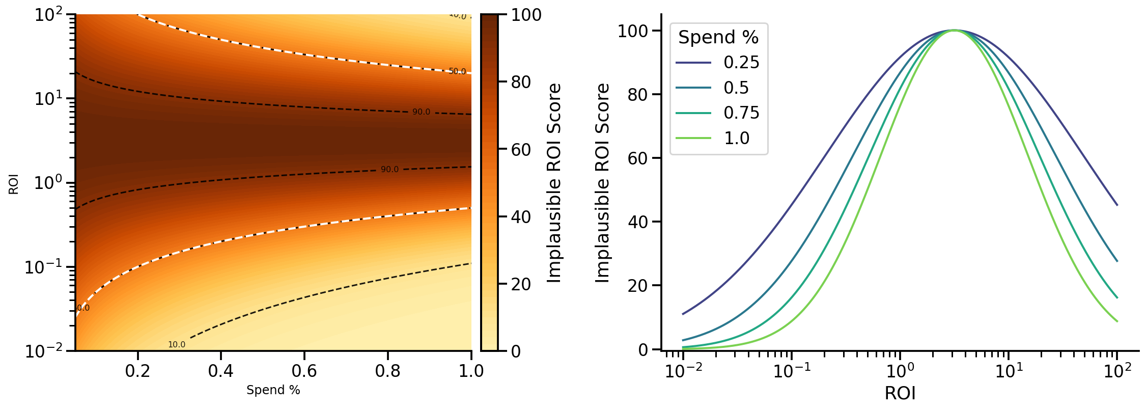
For additional details, see Implausible ROI score in the appendix.
High variance ROI score
The high variance ROI score is a one-sided version of the implausible ROI score based on the width of the ROI posterior credible interval. The score is set to 100 if the spend-weighted relative credible interval is less than 0.5. As the spend-weighted relative credible interval increases, the score decreases.
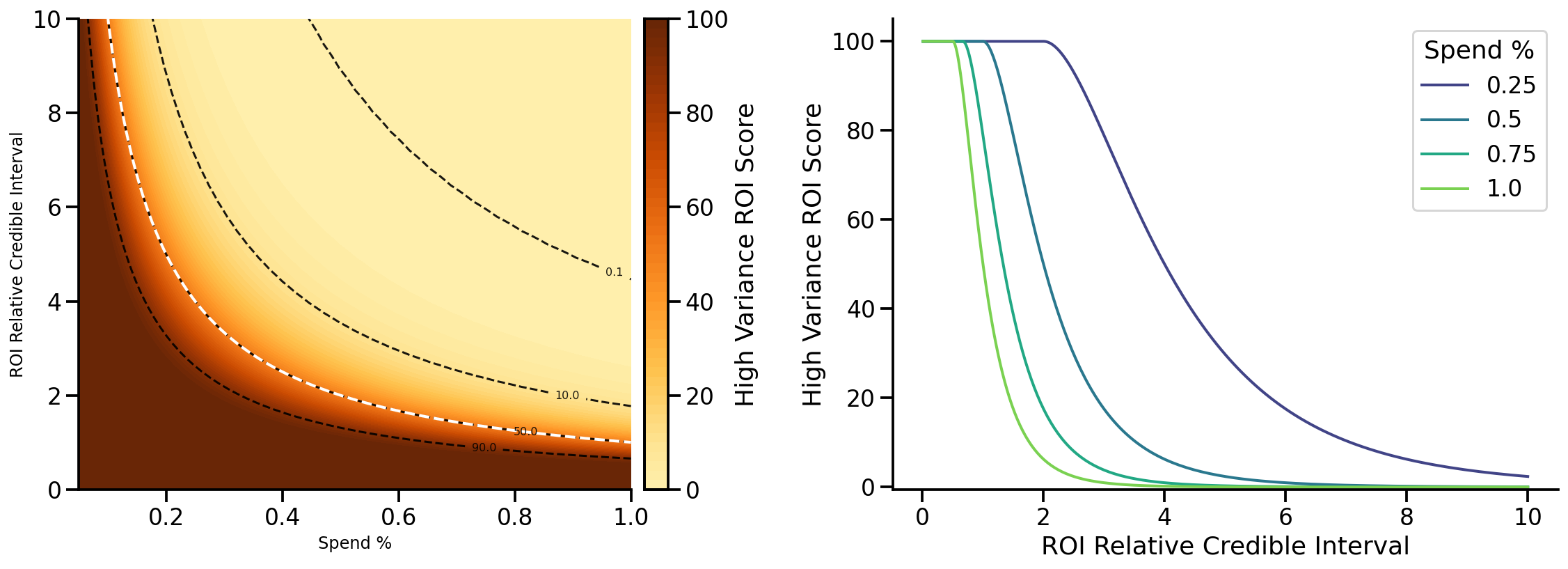
For additional details, see High variance ROI score in the appendix.
Potential bias score
The potential bias score evaluates the maximum correlation between channels and controls. It is defined according to a power relationship based on the maximum correlation (in absolute value) and an exponent.
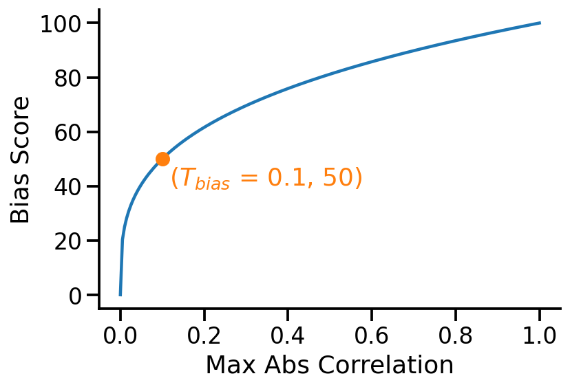
For additional details, see Potential bias score in the appendix.
Understand the model level composite calibration score
The model level composite calibration score is the average of the calibration scores of each channel. Calibrated channels have scores set to 100 in the average, reflecting the fact that they have been calibrated.
If you aren't using CalibrationBuilder but would like to flag channels as
calibrated to accurately compute the model level composite score, you can use
the CalibratedDistribution class directly:
import numpy as np
import tensorflow_probability.substrates.jax as tfp_jax
from meridian.model.calibration import base
from meridian.model import prior_distribution

# Two media channels. The second channel is self-calibrated
distributions = tfp_jax.distributions.LogNormal(
    np.array([0.2, 0.3], dtype=np.float64),
    np.array([0.9, 0.7], dtype=np.float64),
)
roi_m_prior = base.CalibratedDistribution(
    distributions,
    is_calibrated=[False, True],
)
prior = prior_distribution.PriorDistribution(
    roi_m=roi_m_prior,
)
# Pass prior to ModelSpec and continue with modeling
Mathematical appendix
This section describes technical details of the implausible ROI score, high variance ROI score, and potential bias score. For additional details on mathematical notation used below, see the Mathematical notation reference.
Implausible ROI score
Meridian uses a normalized bowl formulation that combines the low ROI and high ROI criteria to prioritize parsimoniousness and user comprehension. This formulation calculates the normalized log distance from the geometric center of the non-flagged region. The steps to compute the score are as follows:
- The geometric center of the low and high thresholds is established.
- The distance from the channel's ROI to this center is calculated relative to the boundaries.
- The resulting score is defined by a bowl shape, where a hyperparameter k defines the steepness of the bowl.
Specifically, let \(z = \log \left(r / M \right)\) be the log distance from geometric center of the low ROI and high ROI thresholds \(M = \sqrt{T_{\text{low_roi}} \cdot T_{\text{high_roi}}} = \sqrt{10}\). Then for any spend percent \(S_{\%}\), the distance from \(M\) to the higher and lower boundary is \(\pm D\) where
\[ D = \log \left(\frac{1}{S_{\%}}\sqrt{\frac{T_{\text{high_roi}}}{T_{\text{low_roi}}}}\right) \]
so that the ratio \(z / D\) defines a normalized log distance to the boundaries. We then define the normalized bowl score as
\[ S_\text{bowl} = 100 \cdot \exp \left( - k \left(\frac{z}{D}\right)^2\right) \]
where \(k\) is a hyperparameter that defines the steepness of the bowl. We select \(k = \log (2)\) so that \(S_\text{bowl} = 1/2\) along the boundaries.
High variance ROI score
The high variance ROI score is a one-sided version of the normalized bowl used in the implausible ROI score. Because the reference point for variance is zero, the standard logarithmic approach used in the Normalized Bowl becomes ill-defined near the reference point.
To resolve this, Meridian uses a normalized half-bowl formulation based on the normalized bowl formulation from the implausible ROI check. This half bowl formulation is a function of the relative credible interval of the posterior: the spend-weighted, normalized, posterior ROI 80th percentile credible interval relative to the width of the 80th percentile credible interval of the Meridian default ROI prior (LogNormal(0.2, 0.9)). The credible interval is taken to be the highest density interval.
A reference ideal region is defined for the relative credible interval: if the spend-weighted relative credible interval width is less than 0.5, the score is set to 100. As the relative credible interval increases beyond the ideal point, the score decreases following the half-bowl curve. Specifically, for every value of \(S_{\%} \cdot \text{RCI} < T_{\text{ideal}} = 0.5\), where RCI is the posterior ROI relative credible interval, the score is set to 100:
\[ S_{\text{half_bowl}}(\text{RCI}, S_{\%}) = \begin{cases} 100, & S_{\%} \cdot \text{RCI} \le T_{\text{ideal}} \\ 100 \cdot \exp\left(-k \left(\frac{\ln(S_{\%} \cdot \text{RCI}/T_{\text{ideal}})}{\ln(T_{\text{high_variance}}/T_{\text{ideal}})}\right)^2\right), & S_{\%} \cdot \text{RCI} > T_{\text{ideal}} \end{cases} \]
As in the implausible ROI score, \(k = \log(2)\) is used.
Potential bias score
The potential bias score is a function of the maximum correlation between channels and controls. It is defined according to a power relationship based on the maximum correlation (in absolute value) and an exponent. The exponent is explicitly selected so that the potential bias score equals exactly 50 at the correlation threshold of 0.1.
- The penalty rises sharply from a maximum correlation of 0.0 to 0.1, where the score evaluates to 50.
- After passing 0.1, the score gradually increases until it hits its maximum penalty at a correlation of 100.
Specifically, the potential bias score has a power relationship:
\[ C_\text{bias} = 100 \cdot \left(b_\text{max}\right) ^ p, \]
where \(b_\text{max}\) is the maximum absolute correlation for the given channel between its execution and any control variable across all geos:
\[ b_\text{max} = \max_{j, g} |\text{corr}_t (E_{g,t,i}, z^{[C]}_{g,t,j}) | \]
with \(E_{g,t,i}\) being \(x^{[M]}_{g,t,i}\) for paid media channels or \(r^{[RF]}_{g,t,i} \cdot f^{[RF]}_{g,t,i}\) for paid reach and frequency channels. Here, \(p\) is an exponent. \(p=\log(0.5) / \log(T_\text{bias})\) is selected so that the potential bias score is 50 at the threshold of the potential bias check, \(T_\text{bias} = 0.1\).