Page Summary
-
Text classification models are selected based on the ratio of samples to words, utilizing either n-gram (for low ratios) or sequence models (for high ratios).
-
Model architecture varies depending on the classification type (binary or multi-class), influencing the last layer's activation function and loss function.
-
N-gram models, like MLPs, process tokens independently, while sequence models, such as sepCNNs, consider word order and may utilize pre-trained embeddings.
-
Model training involves minimizing prediction error by adjusting network weights using an optimizer, with performance tracked via metrics and loss functions.
-
Hyperparameters like learning rate, epochs, and batch size are tuned during training, potentially employing early stopping to prevent overfitting.
In this section, we will work towards building, training and evaluating our
model. In Step 3, we
chose to use either an n-gram model or sequence model, using our S/W ratio.
Now, it’s time to write our classification algorithm and train it. We will use
TensorFlow with the
tf.keras
API for this.
Building machine learning models with Keras is all about assembling together layers, data-processing building blocks, much like we would assemble Lego bricks. These layers allow us to specify the sequence of transformations we want to perform on our input. As our learning algorithm takes in a single text input and outputs a single classification, we can create a linear stack of layers using the Sequential model API.
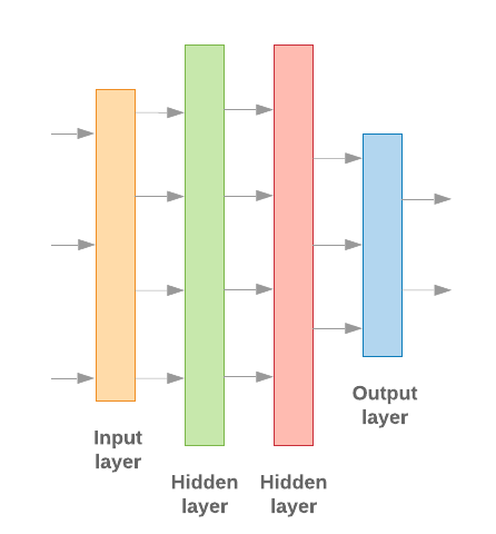
Figure 9: Linear stack of layers
The input layer and the intermediate layers will be constructed differently, depending on whether we’re building an n-gram or a sequence model. But irrespective of model type, the last layer will be the same for a given problem.
Constructing the Last Layer
When we have only 2 classes (binary classification), our model should output a
single probability score. For instance, outputting 0.2 for a given input sample
means “20% confidence that this sample is in the first class (class 1), 80% that
it is in the second class (class 0).” To output such a probability score, the
activation function
of the last layer should be a
sigmoid function,
and the
loss function
used to train the model should be
binary cross-entropy.
(See Figure 10, left).
When there are more than 2 classes (multi-class classification), our model
should output one probability score per class. The sum of these scores should be
1. For instance, outputting {0: 0.2, 1: 0.7, 2: 0.1} means “20% confidence that
this sample is in class 0, 70% that it is in class 1, and 10% that it is in
class 2.” To output these scores, the activation function of the last layer
should be softmax, and the loss function used to train the model should be
categorical cross-entropy. (See Figure 10, right).
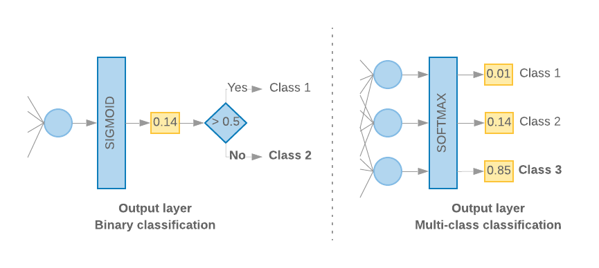
Figure 10: Last layer
The following code defines a function that takes the number of classes as input, and outputs the appropriate number of layer units (1 unit for binary classification; otherwise 1 unit for each class) and the appropriate activation function:
def _get_last_layer_units_and_activation(num_classes):
    """Gets the # units and activation function for the last network layer.

    # Arguments
        num_classes: int, number of classes.

    # Returns
        units, activation values.
    """
    if num_classes == 2:
        activation = 'sigmoid'
        units = 1
    else:
        activation = 'softmax'
        units = num_classes
    return units, activation
The following two sections walk through the creation of the remaining model layers for n-gram models and sequence models.
When the S/W ratio is small, we’ve found that n-gram models perform better
than sequence models. Sequence models are better when there are a large number
of small, dense vectors. This is because embedding relationships are learned in
dense space, and this happens best over many samples.
Build n-gram model [Option A]
We refer to models that process the tokens independently (not taking into account word order) as n-gram models. Simple multi-layer perceptrons (including logistic regression gradient boosting machines, and support vector machines models) all fall under this category; they cannot use any information about text ordering.
We compared the performance of some of the n-gram models mentioned above and observed that multi-layer perceptrons (MLPs) typically perform better than other options. MLPs are simple to define and understand, provide good accuracy, and require relatively little computation.
The following code defines a two-layer MLP model in tf.keras, adding a couple of Dropout layers for regularization to prevent overfitting to training samples.
from tensorflow.python.keras import models
from tensorflow.python.keras.layers import Dense
from tensorflow.python.keras.layers import Dropout

def mlp_model(layers, units, dropout_rate, input_shape, num_classes):
    """Creates an instance of a multi-layer perceptron model.

    # Arguments
        layers: int, number of `Dense` layers in the model.
        units: int, output dimension of the layers.
        dropout_rate: float, percentage of input to drop at Dropout layers.
        input_shape: tuple, shape of input to the model.
        num_classes: int, number of output classes.

    # Returns
        An MLP model instance.
    """
    op_units, op_activation = _get_last_layer_units_and_activation(num_classes)
    model = models.Sequential()
    model.add(Dropout(rate=dropout_rate, input_shape=input_shape))

    for _ in range(layers-1):
        model.add(Dense(units=units, activation='relu'))
        model.add(Dropout(rate=dropout_rate))

    model.add(Dense(units=op_units, activation=op_activation))
    return model
Build sequence model [Option B]
We refer to models that can learn from the adjacency of tokens as sequence models. This includes CNN and RNN classes of models. Data is pre-processed as sequence vectors for these models.
Sequence models generally have a larger number of parameters to learn. The first layer in these models is an embedding layer, which learns the relationship between the words in a dense vector space. Learning word relationships works best over many samples.
Words in a given dataset are most likely not unique to that dataset. We can thus learn the relationship between the words in our dataset using other dataset(s). To do so, we can transfer an embedding learned from another dataset into our embedding layer. These embeddings are referred to as pre-trained embeddings. Using a pre-trained embedding gives the model a head start in the learning process.
There are pre-trained embeddings available that have been trained using large corpora, such as GloVe. GloVe has been trained on multiple corpora (primarily Wikipedia). We tested training our sequence models using a version of GloVe embeddings and observed that if we froze the weights of the pre-trained embeddings and trained just the rest of the network, the models did not perform well. This could be because the context in which the embedding layer was trained might have been different from the context in which we were using it.
GloVe embeddings trained on Wikipedia data may not align with the language patterns in our IMDb dataset. The relationships inferred may need some updating—i.e., the embedding weights may need contextual tuning. We do this in two stages:
In the first run, with the embedding layer weights frozen, we allow the rest of the network to learn. At the end of this run, the model weights reach a state that is much better than their uninitialized values. For the second run, we allow the embedding layer to also learn, making fine adjustments to all weights in the network. We refer to this process as using a fine-tuned embedding.
Fine-tuned embeddings yield better accuracy. However, this comes at the expense of increased compute power required to train the network. Given a sufficient number of samples, we could do just as well learning an embedding from scratch. We observed that for
S/W > 15K, starting from scratch effectively yields about the same accuracy as using fine-tuned embedding.
We compared different sequence models such as CNN, sepCNN, RNN (LSTM & GRU), CNN-RNN, and stacked RNN, varying the model architectures. We found that sepCNNs, a convolutional network variant that is often more data-efficient and compute-efficient, perform better than the other models.
The following code constructs a four-layer sepCNN model:
from tensorflow.python.keras import models
from tensorflow.python.keras import initializers
from tensorflow.python.keras import regularizers

from tensorflow.python.keras.layers import Dense
from tensorflow.python.keras.layers import Dropout
from tensorflow.python.keras.layers import Embedding
from tensorflow.python.keras.layers import SeparableConv1D
from tensorflow.python.keras.layers import MaxPooling1D
from tensorflow.python.keras.layers import GlobalAveragePooling1D

def sepcnn_model(blocks,
                 filters,
                 kernel_size,
                 embedding_dim,
                 dropout_rate,
                 pool_size,
                 input_shape,
                 num_classes,
                 num_features,
                 use_pretrained_embedding=False,
                 is_embedding_trainable=False,
                 embedding_matrix=None):
    """Creates an instance of a separable CNN model.

    # Arguments
        blocks: int, number of pairs of sepCNN and pooling blocks in the model.
        filters: int, output dimension of the layers.
        kernel_size: int, length of the convolution window.
        embedding_dim: int, dimension of the embedding vectors.
        dropout_rate: float, percentage of input to drop at Dropout layers.
        pool_size: int, factor by which to downscale input at MaxPooling layer.
        input_shape: tuple, shape of input to the model.
        num_classes: int, number of output classes.
        num_features: int, number of words (embedding input dimension).
        use_pretrained_embedding: bool, true if pre-trained embedding is on.
        is_embedding_trainable: bool, true if embedding layer is trainable.
        embedding_matrix: dict, dictionary with embedding coefficients.

    # Returns
        A sepCNN model instance.
    """
    op_units, op_activation = _get_last_layer_units_and_activation(num_classes)
    model = models.Sequential()

    # Add embedding layer. If pre-trained embedding is used add weights to the
    # embeddings layer and set trainable to input is_embedding_trainable flag.
    if use_pretrained_embedding:
        model.add(Embedding(input_dim=num_features,
                            output_dim=embedding_dim,
                            input_length=input_shape[0],
                            weights=[embedding_matrix],
                            trainable=is_embedding_trainable))
    else:
        model.add(Embedding(input_dim=num_features,
                            output_dim=embedding_dim,
                            input_length=input_shape[0]))

    for _ in range(blocks-1):
        model.add(Dropout(rate=dropout_rate))
        model.add(SeparableConv1D(filters=filters,
                                  kernel_size=kernel_size,
                                  activation='relu',
                                  bias_initializer='random_uniform',
                                  depthwise_initializer='random_uniform',
                                  padding='same'))
        model.add(MaxPooling1D(pool_size=pool_size))

    model.add(SeparableConv1D(filters=filters * 2,
                              kernel_size=kernel_size,
                              activation='relu',
                              bias_initializer='random_uniform',
                              depthwise_initializer='random_uniform',
                              padding='same'))
    model.add(GlobalAveragePooling1D())
    model.add(Dropout(rate=dropout_rate))
    model.add(Dense(op_units, activation=op_activation))
    return model
Train Your Model
Now that we have constructed the model architecture, we need to train the model. Training involves making a prediction based on the current state of the model, calculating how incorrect the prediction is, and updating the weights or parameters of the network to minimize this error and make the model predict better. We repeat this process until our model has converged and can no longer learn. There are three key parameters to be chosen for this process (See Table 2.)
- Metric: How to measure the performance of our model using a metric. We used accuracy as the metric in our experiments.
- Loss function: A function that is used to calculate a loss value that the training process then attempts to minimize by tuning the network weights. For classification problems, cross-entropy loss works well.
- Optimizer: A function that decides how the network weights will be updated based on the output of the loss function. We used the popular Adam optimizer in our experiments.
In Keras, we can pass these learning parameters to a model using the compile method.
Table 2: Learning parameters
| Learning parameter | Value |
|---|---|
| Metric | accuracy |
| Loss function - binary classification | binary_crossentropy |
| Loss function - multi class classification | sparse_categorical_crossentropy |
| Optimizer | adam |
The actual training happens using the
fit method.
Depending on the size of your
dataset, this is the method in which most compute cycles will be spent. In each
training iteration, batch_size number of samples from your training data are
used to compute the loss, and the weights are updated once, based on this value.
The training process completes an epoch once the model has seen the entire
training dataset. At the end of each epoch, we use the validation dataset to
evaluate how well the model is learning. We repeat training using the dataset
for a predetermined number of epochs. We may optimize this by stopping early,
when the validation accuracy stabilizes between consecutive epochs, showing that
the model is not training anymore.
| Training hyperparameter | Value |
|---|---|
| Learning rate | 1e-3 |
| Epochs | 1000 |
| Batch size | 512 |
| Early stopping | parameter: val_loss, patience: 1 |
Table 3: Training hyperparameters
The following Keras code implements the training process using the parameters chosen in the Tables 2 & 3 above:
def train_ngram_model(data,
                      learning_rate=1e-3,
                      epochs=1000,
                      batch_size=128,
                      layers=2,
                      units=64,
                      dropout_rate=0.2):
    """Trains n-gram model on the given dataset.

    # Arguments
        data: tuples of training and test texts and labels.
        learning_rate: float, learning rate for training model.
        epochs: int, number of epochs.
        batch_size: int, number of samples per batch.
        layers: int, number of `Dense` layers in the model.
        units: int, output dimension of Dense layers in the model.
        dropout_rate: float: percentage of input to drop at Dropout layers.

    # Raises
        ValueError: If validation data has label values which were not seen
            in the training data.
    """
    # Get the data.
    (train_texts, train_labels), (val_texts, val_labels) = data

    # Verify that validation labels are in the same range as training labels.
    num_classes = explore_data.get_num_classes(train_labels)
    unexpected_labels = [v for v in val_labels if v not in range(num_classes)]
    if len(unexpected_labels):
        raise ValueError('Unexpected label values found in the validation set:'
                         ' {unexpected_labels}. Please make sure that the '
                         'labels in the validation set are in the same range '
                         'as training labels.'.format(
                             unexpected_labels=unexpected_labels))

    # Vectorize texts.
    x_train, x_val = vectorize_data.ngram_vectorize(
        train_texts, train_labels, val_texts)

    # Create model instance.
    model = build_model.mlp_model(layers=layers,
                                  units=units,
                                  dropout_rate=dropout_rate,
                                  input_shape=x_train.shape[1:],
                                  num_classes=num_classes)

    # Compile model with learning parameters.
    if num_classes == 2:
        loss = 'binary_crossentropy'
    else:
        loss = 'sparse_categorical_crossentropy'
    optimizer = tf.keras.optimizers.Adam(lr=learning_rate)
    model.compile(optimizer=optimizer, loss=loss, metrics=['acc'])

    # Create callback for early stopping on validation loss. If the loss does
    # not decrease in two consecutive tries, stop training.
    callbacks = [tf.keras.callbacks.EarlyStopping(
        monitor='val_loss', patience=2)]

    # Train and validate model.
    history = model.fit(
            x_train,
            train_labels,
            epochs=epochs,
            callbacks=callbacks,
            validation_data=(x_val, val_labels),
            verbose=2,  # Logs once per epoch.
            batch_size=batch_size)

    # Print results.
    history = history.history
    print('Validation accuracy: {acc}, loss: {loss}'.format(
            acc=history['val_acc'][-1], loss=history['val_loss'][-1]))

    # Save model.
    model.save('IMDb_mlp_model.h5')
    return history['val_acc'][-1], history['val_loss'][-1]
Please find code examples for training the sequence model here.