嵌入欄位可做為迴歸的特徵輸入/預測值,與分類的用法相同。
在本教學課程中,我們將瞭解如何使用 64D 嵌入欄位層做為輸入內容,進行多重迴歸分析,預測地表生物量 (AGB)。
NASA 的全球生態系統動態調查 (GEDI) 計畫會沿著地面橫斷面收集 LIDAR 測量結果,空間解析度為 30 公尺,間隔為 60 公尺。我們會使用 GEDI L4A 地上生物質密度光柵資料集,其中包含地上生物質密度 (AGBD) 的點估計值,這些值將做為迴歸模型中的預測變數。
選取區域
首先,請定義感興趣的區域。在本教學課程中,我們將選取印度西高止山脈的某個區域,並將多邊形定義為幾何變數。或者,您也可以使用程式碼編輯器中的繪圖工具,在感興趣的區域周圍繪製多邊形,並將其儲存為「匯入」中的幾何變數。我們也會使用衛星底圖,方便您找出植被區域。
var geometry = ee.Geometry.Polygon([[
  [74.322, 14.981],
  [74.322, 14.765],
  [74.648, 14.765],
  [74.648, 14.980]
]]);

// Use the satellite basemap
Map.setOptions('SATELLITE');
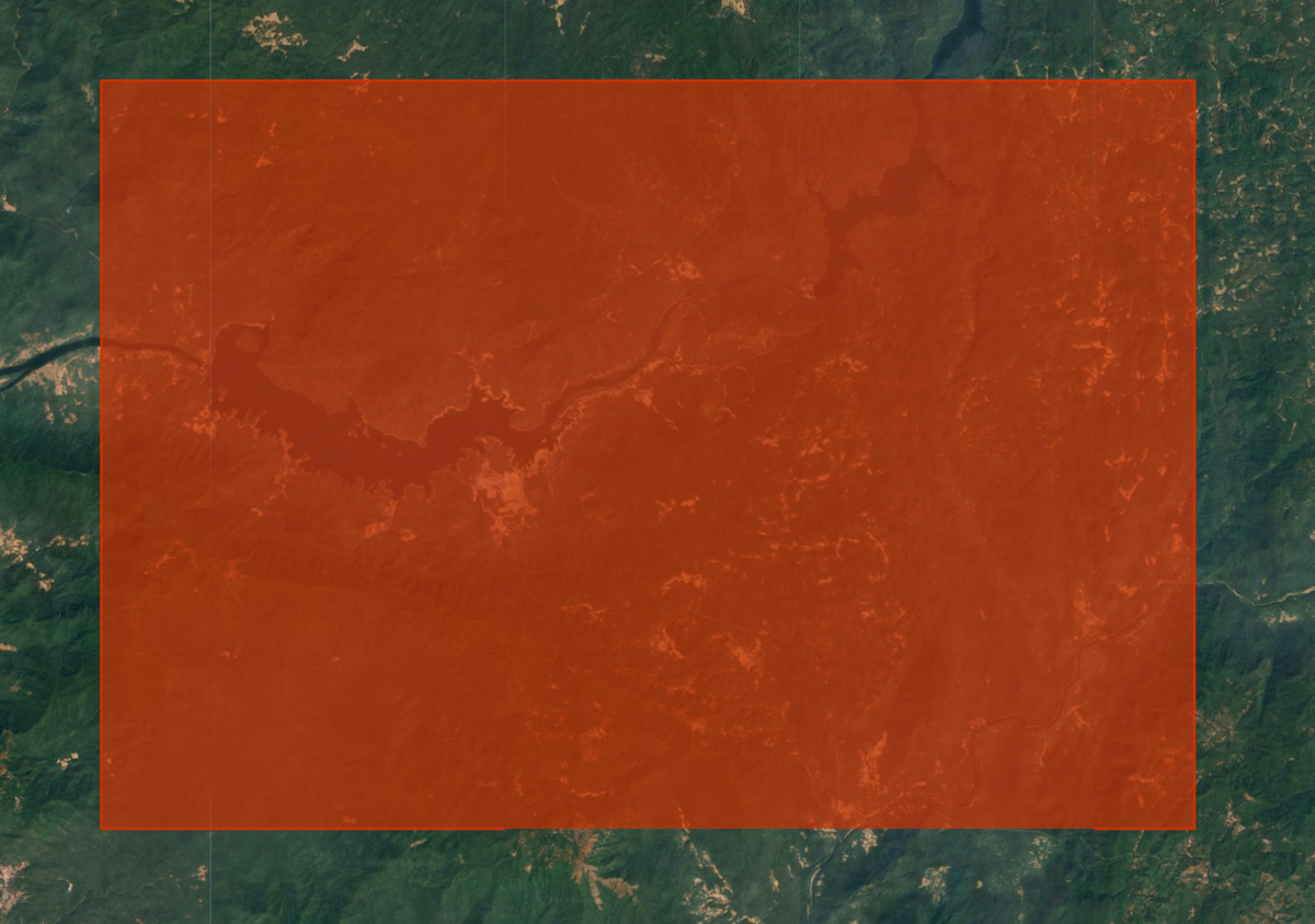
圖:選取地上生物量預測的感興趣區域
選取時間範圍
選擇要執行迴歸的年份。請注意,衛星嵌入內容是以年度為間隔匯總,因此我們定義的期間為整年。
var startDate = ee.Date.fromYMD(2022, 1, 1);
var endDate = startDate.advance(1, 'year');
準備衛星嵌入資料集
64 波段的衛星嵌入式圖片會做為迴歸的預測因子。我們載入 Satellite Embedding 資料集,並篩選所選年份和區域的圖片。
var embeddings = ee.ImageCollection('GOOGLE/SATELLITE_EMBEDDING/V1/ANNUAL');

var embeddingsFiltered = embeddings
  .filter(ee.Filter.date(startDate, endDate))
  .filter(ee.Filter.bounds(geometry));
衛星嵌入圖片會劃分成圖塊,並以圖塊的 UTM 區域投影方式提供。因此,我們會取得多個涵蓋感興趣區域的衛星嵌入式地圖圖塊。如要取得單一圖片,我們需要將這些圖片拼接在一起。在 Earth Engine 中,輸入圖片的影像拼接會指派預設投影,也就是 WGS84,比例為 1 度。我們會在教學課程稍後彙整並重新投影這個鑲嵌,因此保留原始投影很有幫助。我們可以從其中一個圖塊擷取投影資訊,並使用 setDefaultProjection() 函式在馬賽克上設定該資訊。
// Extract the projection of the first band of the first image
var embeddingsProjection = ee.Image(embeddingsFiltered.first()).select(0).projection();

// Set the projection of the mosaic to the extracted projection
var embeddingsImage = embeddingsFiltered.mosaic()
  .setDefaultProjection(embeddingsProjection);
準備 GEDI L4A 鑲嵌
由於 GEDI 生物特徵估計值將用於訓練迴歸模型,因此請務必先篩除無效或不可靠的 GEDI 資料,再加以使用。我們會套用多個遮罩,移除可能錯誤的測量結果。
- 移除所有不符合品質規定的測量值 (l4_quality_flag = 0 且 degrade_flag > 0)
- 移除所有相對誤差較高的測量結果 ('agbd_se' / 'agbd' > 50%)
- 根據 Copernicus GLO-30 數位高程模式 (DEM),移除坡度大於 30% 的所有測量結果
最後,我們選取感興趣時間範圍和區域的所有剩餘測量結果,並建立影像拼接。
var gedi = ee.ImageCollection('LARSE/GEDI/GEDI04_A_002_MONTHLY');
// Function to select the highest quality GEDI data
var qualityMask = function(image) {
  return image.updateMask(image.select('l4_quality_flag').eq(1))
      .updateMask(image.select('degrade_flag').eq(0));
};

// Function to mask unreliable GEDI measurements
// with a relative standard error > 50%
// agbd_se / agbd > 0.5
var errorMask = function(image) {
  var relative_se = image.select('agbd_se')
    .divide(image.select('agbd'));
  return image.updateMask(relative_se.lte(0.5));
};

// Function to mask GEDI measurements on slopes > 30%

var slopeMask = function(image) {
  // Use Copernicus GLO-30 DEM for calculating slope
  var glo30 = ee.ImageCollection('COPERNICUS/DEM/GLO30');

  var glo30Filtered = glo30
    .filter(ee.Filter.bounds(geometry))
    .select('DEM');

  // Extract the projection
  var demProj = glo30Filtered.first().select(0).projection();

  // The dataset consists of individual images
  // Create a mosaic and set the projection
  var elevation = glo30Filtered.mosaic().rename('dem')
    .setDefaultProjection(demProj);

  // Compute the slope
  var slope = ee.Terrain.slope(elevation);

  return image.updateMask(slope.lt(30));
};

var gediFiltered = gedi
  .filter(ee.Filter.date(startDate, endDate))
  .filter(ee.Filter.bounds(geometry));

var gediProjection = ee.Image(gediFiltered.first())
  .select('agbd').projection();

var gediProcessed = gediFiltered
  .map(qualityMask)
  .map(errorMask)
  .map(slopeMask);

var gediMosaic = gediProcessed.mosaic()
  .select('agbd').setDefaultProjection(gediProjection);

// Visualize the GEDI Mosaic
var gediVis = {
  min: 0,
  max: 200,
  palette: ['#edf8fb', '#b2e2e2', '#66c2a4', '#2ca25f', '#006d2c'],
  bands: ['agbd']
};

Map.addLayer(gediMosaic, gediVis, 'GEDI L4A (Filtered)', false);
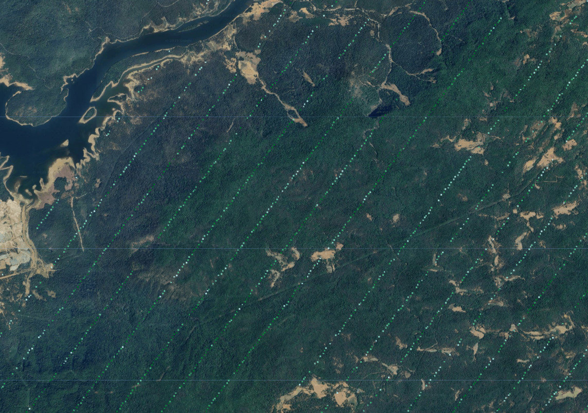
圖:準備好的 GEDI 生物量觀測資料
重新取樣及匯總輸入內容
在對像素取樣以訓練迴歸模型前,我們會重新取樣並重新投影輸入內容至相同的像素格線。GEDI 測量的水平準確度為 +/- 9 公尺。將 GEDI AGB 值與 Satellite 嵌入像素比對時,這會造成問題。為解決這個問題,我們會重新取樣並匯總所有輸入圖片,以原始像素的平均值建立較大的像素格線。這也有助於從資料中移除雜訊,並建構更完善的機器學習模型。
// Choose the grid size and projection
var gridScale = 100;
var gridProjection = ee.Projection('EPSG:3857')
  .atScale(gridScale);

// Create a stacked image with predictor and predicted variables
var stacked = embeddingsImage.addBands(gediMosaic);

//  Set the resampling mode
var stacked = stacked.resample('bilinear');

// Aggregate pixels with 'mean' statistics
var stackedResampled = stacked
  .reduceResolution({
    reducer: ee.Reducer.mean(),
    maxPixels: 1024
  })
  .reproject({
    crs: gridProjection
});

// As larger GEDI pixels contain masked original
// pixels, it has a transparency mask.
// We update the mask to remove the transparency
var stackedResampled = stackedResampled
  .updateMask(stackedResampled.mask().gt(0));
重新投影和匯總像素是耗費資源的作業,因此建議您匯出產生的堆疊影像做為資產,並在後續步驟中使用預先計算的影像。這樣一來,處理大型區域時,就能避免發生計算逾時或超出使用者記憶體限制錯誤。
// Replace this with your asset folder
// The folder must exist before exporting
var exportFolder = 'projects/spatialthoughts/assets/satellite_embedding/';
var mosaicExportImage = 'gedi_mosaic';
var mosaicExportImagePath = exportFolder + mosaicExportImage;
Export.image.toAsset({
  image: stackedResampled.clip(geometry),
  description: 'GEDI_Mosaic_Export',
  assetId: mosaicExportImagePath,
  region: geometry,
  scale: gridScale,
  maxPixels: 1e10
});
啟動匯出工作,並等待工作完成。完成後,我們匯入資產並繼續建構模型。
// Use the exported asset
var stackedResampled = ee.Image(mosaicExportImagePath);
擷取訓練特徵
我們已準備好輸入資料,可供擷取訓練特徵。我們在迴歸模型中,會使用衛星嵌入帶做為依變數 (預測因子),並使用 GEDI AGBD 值做為自變數 (預測值)。我們可以擷取每個像素的重合值,並準備訓練資料集。我們的 GEDI 圖片大多經過遮蓋,只有一小部分像素含有值。如果使用 sample(),則會傳回大部分為空的值。為解決這個問題,我們從 GEDI 遮罩建立類別頻帶,並使用 stratifiedSample() 確保從非遮罩像素取樣。
var predictors = embeddingsImage.bandNames();
var predicted = gediMosaic.bandNames().get(0);
print('predictors', predictors);
print('predicted', predicted);

var predictorImage = stackedResampled.select(predictors);
var predictedImage = stackedResampled.select([predicted]);

var classMask = predictedImage.mask().toInt().rename('class');

var numSamples = 1000;

// We set classPoints to [0, numSamples]
// This will give us 0 points for class 0 (masked areas)
// and numSample points for class 1 (non-masked areas)
var training = stackedResampled.addBands(classMask)
  .stratifiedSample({
    numPoints: numSamples,
    classBand: 'class',
    region: geometry,
    scale: gridScale,
    classValues: [0, 1],
    classPoints: [0, numSamples],
    dropNulls: true,
    tileScale: 16,
});

print('Number of Features Extracted', training.size());
print('Sample Training Feature', training.first());
訓練迴歸模型
我們現在已做好準備,可以開始訓練模型了。Earth Engine 中的許多分類器都可用於分類和迴歸工作。由於我們要預測數值 (而非類別),因此可以將分類器設為在 REGRESSION 模式下執行,並使用訓練資料進行訓練。模型訓練完成後,我們可以比較模型的預測值與輸入值,並計算均方根誤差 (rmse) 和相關係數 r^2,藉此檢查模型的效能。
// Use the RandomForest classifier and set the
// output mode to REGRESSION
var model = ee.Classifier.smileRandomForest(50)
  .setOutputMode('REGRESSION')
  .train({
    features: training,
    classProperty: predicted,
    inputProperties: predictors
  });

// Get model's predictions for training samples
var predicted = training.classify({
  classifier: model,
  outputName: 'agbd_predicted'
});

// Calculate RMSE
var calculateRmse = function(input) {
    var observed = ee.Array(
      input.aggregate_array('agbd'));
    var predicted = ee.Array(
      input.aggregate_array('agbd_predicted'));
    var rmse = observed.subtract(predicted).pow(2)
      .reduce('mean', [0]).sqrt().get([0]);
    return rmse;
};
var rmse = calculateRmse(predicted);
print('RMSE', rmse);

// Create a plot of observed vs. predicted values
var chart = ui.Chart.feature.byFeature({
  features: predicted.select(['agbd', 'agbd_predicted']),
  xProperty: 'agbd',
  yProperties: ['agbd_predicted'],
}).setChartType('ScatterChart')
  .setOptions({
    title: 'Aboveground Biomass Density (Mg/Ha)',
    dataOpacity: 0.8,
    hAxis: {'title': 'Observed'},
    vAxis: {'title': 'Predicted'},
    legend: {position: 'right'},
    series: {
      0: {
        visibleInLegend: false,
        color: '#525252',
        pointSize: 3,
        pointShape: 'triangle',
      },
    },
    trendlines: {
      0: {
        type: 'linear',
        color: 'black',
        lineWidth: 1,
        pointSize: 0,
        labelInLegend: 'Linear Fit',
        visibleInLegend: true,
        showR2: true
      }
    },
    chartArea: {left: 100, bottom: 100, width: '50%'},

});
print(chart);
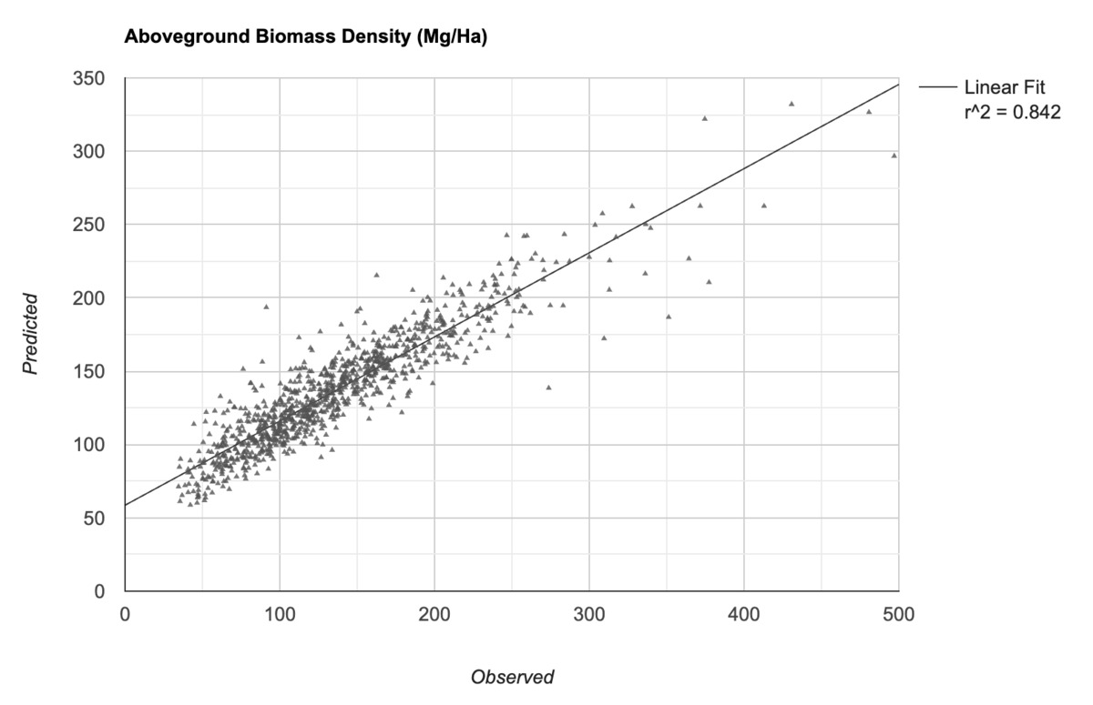
圖:觀測到的 AGBD 值與模型預測的 AGBD 值
為不明值產生預測
對模型感到滿意後,我們就能使用訓練好的模型,根據含有預測帶的圖片,在未知位置生成預測結果。
// We set the band name of the output image as 'agbd'
var predictedImage = stackedResampled.classify({
  classifier: model,
  outputName: 'agbd'
});
現在可以匯出圖片,其中包含每個像素的預測 AGBD 值。我們會在下一節使用這項資料,將結果視覺化。
// Replace this with your asset folder
// The folder must exist before exporting
var exportFolder = 'projects/spatialthoughts/assets/satellite_embedding/';
var predictedExportImage = 'predicted_agbd';
var predictedExportImagePath = exportFolder + predictedExportImage;

Export.image.toAsset({
  image: predictedImage.clip(geometry),
  description: 'Predicted_Image_Export',
  assetId: predictedExportImagePath,
  region: geometry,
  scale: gridScale,
  maxPixels: 1e10
});
啟動匯出工作,並等待工作完成。完成後,我們會匯入資產並將結果視覺化。
var predictedImage = ee.Image(predictedExportImagePath);

// Visualize the image
var gediVis = {
  min: 0,
  max: 200,
  palette: ['#edf8fb', '#b2e2e2', '#66c2a4', '#2ca25f', '#006d2c'],
  bands: ['agbd']
};

Map.addLayer(predictedImage, gediVis, 'Predicted AGBD');
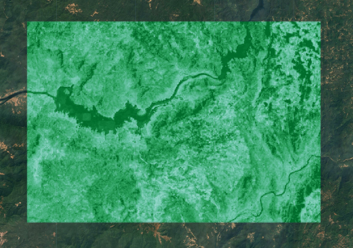
圖:預測的 AGBD。深綠色表示預測的生物質密度較高
預估生物質總量
現在我們已取得圖片中每個像素的預測 AGBD 值,可用於估算該區域的地上生物質 (AGB) 總量。但我們必須先移除所有屬於非植被區域的像素。我們可以運用 ESA WorldCover 土地覆蓋資料集,選取植被像素。
// GEDI data is processed only for certain landcovers
// from Plant Functional Types (PFT) classification
// https://doi.org/10.1029/2022EA002516

// Here we use ESA WorldCover v200 product to
// select landcovers representing vegetated areas
var worldcover = ee.ImageCollection('ESA/WorldCover/v200').first();

// Aggregate pixels to the same grid as other dataset
// with 'mode' value.
// i.e. The landcover with highest occurrence within the grid
var worldcoverResampled = worldcover
  .reduceResolution({
    reducer: ee.Reducer.mode(),
    maxPixels: 1024
  })
  .reproject({
    crs: gridProjection
});

// Select grids for the following classes
// | Class Name | Value |
// | Forests    | 10    |
// | Shrubland  | 20    |
// | Grassland  | 30    |
// | Cropland   | 40    |
// | Mangroves  | 95    |
var landCoverMask = worldcoverResampled.eq(10)
    .or(worldcoverResampled.eq(20))
    .or(worldcoverResampled.eq(30))
    .or(worldcoverResampled.eq(40))
    .or(worldcoverResampled.eq(95));

var predictedImageMasked = predictedImage
  .updateMask(landCoverMask);
Map.addLayer(predictedImageMasked, gediVis, 'Predicted AGBD (Masked)');
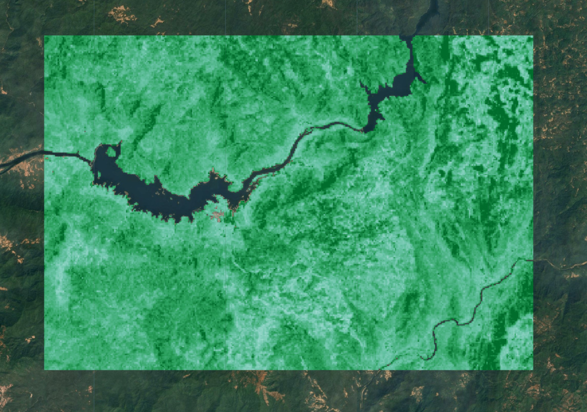
圖:預測的 AGBD,非植被區域已遮蓋
GEDI AGBD 值的單位為每公頃百萬公克 (Mg/ha)。如要取得 AGB 總量,請將每個像素乘以其面積 (以公頃為單位),然後加總這些值。
var pixelAreaHa = ee.Image.pixelArea().divide(10000);
var predictedAgb = predictedImageMasked.multiply(pixelAreaHa);

var stats = predictedAgb.reduceRegion({
  reducer: ee.Reducer.sum(),
  geometry: geometry,
  scale: gridScale,
  maxPixels: 1e10,
  tileScale: 16
});

// Result is a dictionary with key for each band
var totalAgb = stats.getNumber('agbd');

print('Total AGB (Mg)', totalAgb);