
Conditional formatting lets you format cells so that their appearance changes dynamically according to the value they contain, or to values in other cells. There are many possible applications of conditional formatting, including these uses:
- Highlight cells above a certain threshold (for example, using bold text for all transactions over $2,000).
- Format cells so their color varies with their value (for example, applying a more intense red background as the amount over $2,000 increases).
- Dynamically format cells based on the content of other cells (for example, highlighting the address of properties whose "time on market" field is > 90 days).
You can even format cells based on their value and those of other cells. For example, you could format a range of cells based on their value compared to the median value of the range:
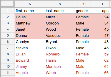
Figure 1. Formatting to highlight values above or below the median age.
In this example, the cells in each row are formatted according to how the value
in their age column compares to the median value of all the ages. Rows whose
age is above the median have red text, and those below the median have a red
background. Two of the rows have a value for age that matches the median age
(48) and these cells receive no special formatting. (For the source code that
creates this conditional formatting, see the Example below.)
Conditional formatting rules
Conditional formatting is expressed using formatting rules. Each spreadsheet stores a list of these rules, and applies them in the same order as they appear in the list. The Google Sheets API lets you add, update, and delete these formatting rules.
Each rule specifies a target range, type of rule, conditions for triggering the rule, and any formatting to apply.
Target range—This can be a single cell, a range of cells, or multiple ranges.
Type of rule—There are two categories of rules:
- Boolean rules apply a format only if specific criteria are met.
- Gradient rules calculate the background color of a cell, based on the value of the cell.
The conditions that are evaluated, and the formats that you can apply, are different for each of these rule types, as detailed in the following sections.
Boolean rules
A
BooleanRule
defines whether to apply a specific format, based on a
BooleanCondition
that evaluates to true or false. A boolean rule takes the form:
{
  "condition": {
    object(BooleanCondition)
  },
  "format": {
    object(CellFormat)
  },
}
The condition can use the built-in
ConditionType,
or it can use a custom formula for more complex evaluations.
Built-in types let you apply formatting according to numeric thresholds,
text comparison, or whether a cell is populated. For example, NUMBER_GREATER
means the cell's value must be greater than the condition's value. Rules are
always evaluated against the target cell.
Custom formula is a special condition type that lets you apply formatting
according to an arbitrary expression, which also allows evaluation of any cell,
not just the target cell. The condition's formula must evaluate to true.
To define the formatting applied by a boolean rule, you use a subset of the
CellFormat
type to define:
- Whether the text in the cell is bold, italic, or strikethrough.
- The text color in the cell.
- The background color of the cell.
Gradient rules
A
GradientRule
defines a range of colors that correspond to a range of values. A gradient rule
takes the form:
{
  "minpoint": {
    object(InterpolationPoint)
  },
  "midpoint": {
    object(InterpolationPoint)
  },
  "maxpoint": {
    object(InterpolationPoint)
  },
}
Each
InterpolationPoint
defines a color and its corresponding value. A set of three points defines a
color gradient.
Manage conditional formatting rules
To create, modify, or delete conditional formatting rules, use the
spreadsheets.batchUpdate
method with the appropriate request type:
Add rules to the list at the given index using the
AddConditionalFormatRuleRequest.Replace or reorder rules in the list at the given index using the
UpdateConditionalFormatRuleRequest.Remove rules from the list at the given index using the
DeleteConditionalFormatRuleRequest.
Example
The following example shows how to create the conditional formatting shown in the screenshot at the top of this page. For additional examples, see the Conditional formatting samples page.