এই পাতায় মেট্রিক্সের পরিভাষা তালিকা রয়েছে। সম্পূর্ণ পরিভাষা তালিকার জন্য এখানে ক্লিক করুন ।
একটি
নির্ভুলতা
সঠিক শ্রেণিবিন্যাস ভবিষ্যদ্বাণীর সংখ্যাকে মোট ভবিষ্যদ্বাণীর সংখ্যা দিয়ে ভাগ করলে যা পাওয়া যায়। অর্থাৎ:
উদাহরণস্বরূপ, যে মডেলটি ৪০টি সঠিক ভবিষ্যদ্বাণী এবং ১০টি ভুল ভবিষ্যদ্বাণী করেছে, তার নির্ভুলতা হবে:
বাইনারি ক্লাসিফিকেশন সঠিক ভবিষ্যদ্বাণী এবং ভুল ভবিষ্যদ্বাণীর বিভিন্ন বিভাগের জন্য নির্দিষ্ট নাম প্রদান করে। সুতরাং, বাইনারি ক্লাসিফিকেশনের জন্য অ্যাকুরেসি সূত্রটি নিম্নরূপ:
যেখানে:
- TP হলো ট্রু পজিটিভের (সঠিক ভবিষ্যদ্বাণীর) সংখ্যা।
- TN হলো ট্রু নেগেটিভের (সঠিক ভবিষ্যদ্বাণীর) সংখ্যা।
- FP হলো ফলস পজিটিভের (ভুল ভবিষ্যদ্বাণীর) সংখ্যা।
- FN হলো ফলস নেগেটিভের (ভুল পূর্বাভাসের) সংখ্যা।
অ্যাক্যুরেসি , প্রিসিশন এবং রিকলের মধ্যে তুলনা ও বৈসাদৃশ্য দেখান।
আরও তথ্যের জন্য মেশিন লার্নিং ক্র্যাশ কোর্সে ‘শ্রেণিবিন্যাস: অ্যাকুরেসি, রিকল, প্রিসিশন এবং সম্পর্কিত মেট্রিকস’ দেখুন।
PR বক্ররেখার নিচের এলাকা
পিআর এইউসি (পিআর কার্ভের নিচের ক্ষেত্রফল) দেখুন।
ROC বক্ররেখার নিচের ক্ষেত্রফল
AUC (ROC কার্ভের নিচের ক্ষেত্রফল) দেখুন।
AUC (ROC বক্ররেখার নিচের ক্ষেত্রফল)
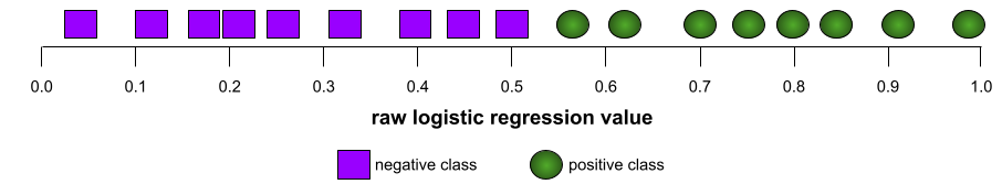
০.০ থেকে ১.০-এর মধ্যে একটি সংখ্যা, যা একটি বাইনারি ক্লাসিফিকেশন মডেলের পজিটিভ ক্লাস থেকে নেগেটিভ ক্লাসকে আলাদা করার ক্ষমতাকে নির্দেশ করে। AUC-এর মান ১.০-এর যত কাছাকাছি হবে, ক্লাসগুলোকে একে অপরের থেকে আলাদা করার ক্ষেত্রে মডেলটির ক্ষমতা তত ভালো হবে।
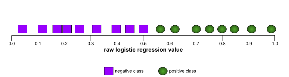
উদাহরণস্বরূপ, নিম্নলিখিত চিত্রটি এমন একটি ক্লাসিফিকেশন মডেল দেখায় যা পজিটিভ ক্লাস (সবুজ ডিম্বাকৃতি) এবং নেগেটিভ ক্লাস (বেগুনি আয়তক্ষেত্র)-কে নিখুঁতভাবে আলাদা করে। এই অবাস্তবভাবে নিখুঁত মডেলটির AUC হলো ১.০:
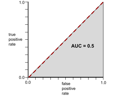
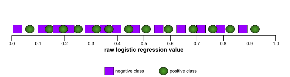
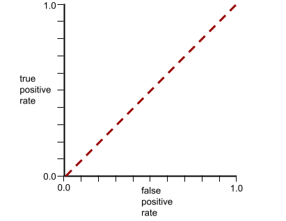
বিপরীতভাবে, নিম্নলিখিত উদাহরণটি এমন একটি ক্লাসিফিকেশন মডেলের ফলাফল দেখাচ্ছে যা এলোমেলো ফলাফল তৈরি করেছে। এই মডেলটির AUC হলো ০.৫:
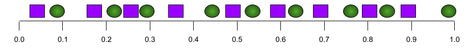
হ্যাঁ, পূর্ববর্তী মডেলটির AUC ০.৫, ০.০ নয়।
বেশিরভাগ মডেলই এই দুটি চরম সীমার মাঝামাঝি কোথাও থাকে। উদাহরণস্বরূপ, নিম্নলিখিত মডেলটি ধনাত্মক ও ঋণাত্মক মানকে কিছুটা আলাদা করে, এবং তাই এর AUC ০.৫ থেকে ১.০-এর মধ্যে থাকে:
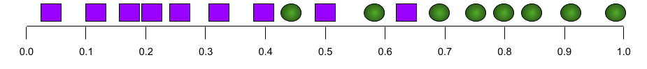
AUC ক্লাসিফিকেশন থ্রেশহোল্ডের জন্য আপনার সেট করা যেকোনো মান উপেক্ষা করে। পরিবর্তে, AUC সমস্ত সম্ভাব্য ক্লাসিফিকেশন থ্রেশহোল্ড বিবেচনা করে।
AUC এবং ROC কার্ভের মধ্যে সম্পর্ক সম্পর্কে জানতে আইকনটিতে ক্লিক করুন।
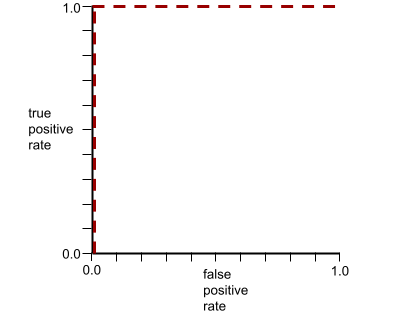
AUC হলো একটি ROC কার্ভের নিচের ক্ষেত্রফল । উদাহরণস্বরূপ, যে মডেলটি পজিটিভ ও নেগেটিভকে নিখুঁতভাবে আলাদা করে, তার ROC কার্ভটি দেখতে নিম্নরূপ:
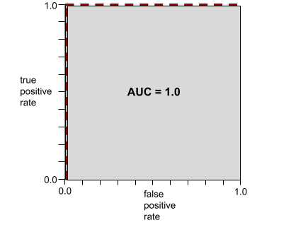
AUC হলো পূর্ববর্তী চিত্রে ধূসর অঞ্চলের ক্ষেত্রফল। এই অস্বাভাবিক ক্ষেত্রে, ক্ষেত্রফলটি হলো ধূসর অঞ্চলের দৈর্ঘ্য (1.0) এবং ধূসর অঞ্চলের প্রস্থ (1.0) এর গুণফল। সুতরাং, 1.0 এবং 1.0 এর গুণফলের ফলে AUC ঠিক 1.0 হয়, যা সর্বোচ্চ সম্ভাব্য AUC স্কোর।
বিপরীতভাবে, যে ক্লাসিফিকেশন মডেলটি ক্লাসগুলোকে একেবারেই আলাদা করতে পারে না, তার ROC কার্ভটি নিম্নরূপ। এই ধূসর অঞ্চলের ক্ষেত্রফল হলো ০.৫।
একটি সাধারণ ROC কার্ভ দেখতে প্রায় নিচের মতো হয়:
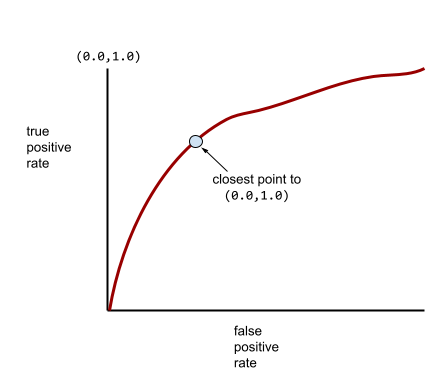
এই বক্ররেখার নিচের ক্ষেত্রফল হাতে-কলমে গণনা করা কষ্টসাধ্য, একারণেই সাধারণত একটি প্রোগ্রাম বেশিরভাগ AUC মান গণনা করে থাকে।
আরও তথ্যের জন্য মেশিন লার্নিং ক্র্যাশ কোর্সে ‘শ্রেণিবিন্যাস: ROC এবং AUC’ দেখুন।
k-তে গড় নির্ভুলতা
একটি মডেলের পারফরম্যান্সকে একটিমাত্র প্রম্পটের উপর সংক্ষিপ্ত করার জন্য ব্যবহৃত একটি মেট্রিক, যা র্যাঙ্ক করা ফলাফল তৈরি করে, যেমন বইয়ের সুপারিশের একটি সংখ্যাযুক্ত তালিকা। k- তে গড় প্রিসিশন হলো, প্রতিটি প্রাসঙ্গিক ফলাফলের জন্য k-তে প্রিসিশন মানগুলোর গড়। সুতরাং, k- তে গড় প্রিসিশনের সূত্রটি হলো:
\[{\text{average precision at k}} = \frac{1}{n} \sum_{i=1}^n {\text{precision at k for each relevant item} } \]
যেখানে:
- \(n\) তালিকায় প্রাসঙ্গিক আইটেমের সংখ্যা।
k-তে স্মরণের সাথে তুলনা করুন।
বি
বেসলাইন
একটি মডেল যা অন্য একটি মডেলের (সাধারণত, আরও জটিল একটি মডেল) কার্যকারিতা তুলনা করার জন্য একটি নির্দেশক হিসেবে ব্যবহৃত হয়। উদাহরণস্বরূপ, একটি লজিস্টিক রিগ্রেশন মডেল একটি ডিপ মডেলের জন্য ভালো বেসলাইন হিসেবে কাজ করতে পারে।
কোনো নির্দিষ্ট সমস্যার ক্ষেত্রে, বেসলাইন মডেল ডেভেলপারদেরকে সেই ন্যূনতম প্রত্যাশিত পারফরম্যান্সের পরিমাণ নির্ধারণ করতে সাহায্য করে, যা একটি নতুন মডেলকে কার্যকর হওয়ার জন্য অর্জন করতে হবে।
বুলিয়ান প্রশ্ন (BoolQ)
হ্যাঁ-না প্রশ্নের উত্তর দেওয়ার ক্ষেত্রে একজন এলএলএম-এর দক্ষতা মূল্যায়নের জন্য একটি ডেটাসেট। ডেটাসেটের প্রতিটি চ্যালেঞ্জের তিনটি উপাদান রয়েছে:
- একটি প্রশ্ন
- এমন একটি অনুচ্ছেদ যা প্রশ্নটির উত্তরের ইঙ্গিত দেয়।
- সঠিক উত্তরটি হলো হ্যাঁ অথবা না ।
উদাহরণস্বরূপ:
- প্রশ্ন : মিশিগানে কি কোনো পারমাণবিক বিদ্যুৎ কেন্দ্র আছে?
- অনুচ্ছেদ : ...তিনটি পারমাণবিক বিদ্যুৎ কেন্দ্র মিশিগানকে তার প্রায় ৩০% বিদ্যুৎ সরবরাহ করে।
- সঠিক উত্তর : হ্যাঁ
গবেষকরা পরিচয় গোপন রেখে একত্রিত করা গুগল সার্চ কোয়েরি থেকে প্রশ্নগুলো সংগ্রহ করেন এবং এরপর তথ্যের ভিত্তি স্থাপনের জন্য উইকিপিডিয়ার পৃষ্ঠা ব্যবহার করেন।
আরও তথ্যের জন্য, BoolQ: Exploring the Surprising Difficulty of Natural Yes/No Questions দেখুন।
BoolQ হলো SuperGLUE এনসেম্বলের একটি উপাদান।
বুলকিউ
বুলিয়ান প্রশ্নসমূহের সংক্ষিপ্ত রূপ।
সি
সিবি
CommitmentBank- এর সংক্ষিপ্ত রূপ।
ক্যারেক্টার এন-গ্রাম এফ-স্কোর (ChrF)
মেশিন ট্রান্সলেশন মডেল মূল্যায়ন করার একটি মেট্রিক। ক্যারেক্টার এন-গ্রাম এফ-স্কোর নির্ধারণ করে যে , রেফারেন্স টেক্সটের এন-গ্রামগুলো একটি এমএল মডেল দ্বারা তৈরি টেক্সটের এন-গ্রামগুলোর সাথে কতটা মিলে যায়।
ক্যারেক্টার এন-গ্রাম এফ-স্কোর ROUGE এবং BLEU পরিবারের মেট্রিকগুলোর অনুরূপ, তবে ব্যতিক্রম হলো:
- ক্যারেক্টার এন-গ্রাম এফ-স্কোর ক্যারেক্টার এন-গ্রামের উপর কাজ করে।
- ROUGE এবং BLEU ওয়ার্ড এন-গ্রাম বা টোকেনের ওপর কাজ করে।
সম্ভাব্য বিকল্পের নির্বাচন (COPA)
একটি পূর্বানুমানের দুটি বিকল্প উত্তরের মধ্যে অপেক্ষাকৃত ভালো উত্তরটি শনাক্ত করতে একটি এলএলএম (LLM) কতটা পারদর্শী, তা মূল্যায়ন করার জন্য একটি ডেটাসেট। ডেটাসেটের প্রতিটি চ্যালেঞ্জ তিনটি উপাদান নিয়ে গঠিত:
- ভিত্তি, যা সাধারণত একটি বিবৃতির পরে একটি প্রশ্ন নিয়ে গঠিত।
- প্রস্তাবনায় উত্থাপিত প্রশ্নের দুটি সম্ভাব্য উত্তর রয়েছে, যার মধ্যে একটি সঠিক এবং অন্যটি ভুল।
- সঠিক উত্তর
উদাহরণস্বরূপ:
- প্রেক্ষাপট: লোকটির পায়ের আঙুল ভেঙে গেছে। এর কারণ কী ছিল?
- সম্ভাব্য উত্তর:
- তার মোজায় একটা ফুটো হয়ে গেল।
- সে তার পায়ের উপর একটি হাতুড়ি ফেলে দিল।
- সঠিক উত্তর: ২
COPA হলো SuperGLUE সমষ্টির একটি উপাদান।
কমিটমেন্ট ব্যাংক (সিবি)
কোনো অনুচ্ছেদের লেখক সেই অনুচ্ছেদের মধ্যে থাকা একটি নির্দিষ্ট বাক্যাংশে বিশ্বাস করেন কি না, তা নির্ধারণে একজন এলএলএম-এর দক্ষতা মূল্যায়নের জন্য একটি ডেটাসেট। ডেটাসেটের প্রতিটি এন্ট্রিতে রয়েছে:
- একটি অনুচ্ছেদ
- সেই অনুচ্ছেদের মধ্যে একটি লক্ষ্য ধারা
- একটি বুলিয়ান মান যা নির্দেশ করে যে অনুচ্ছেদটির লেখক লক্ষ্য বাক্যাংশটিতে বিশ্বাস করেন কিনা।
উদাহরণস্বরূপ:
- আর্টেমিসের হাসি শুনতে কী মজা ! ও তো খুবই গম্ভীর একটা বাচ্চা। আমি তো জানতামই না ওর রসবোধ আছে।
- লক্ষ্য বাক্যাংশ: তার রসবোধ ছিল
- বুলিয়ান : True, যার অর্থ লেখক লক্ষ্য ধারাটি বিশ্বাস করেন
CommitmentBank হলো SuperGLUE এনসেম্বলের একটি উপাদান।
কোপা
সম্ভাব্য বিকল্প নির্বাচনের সংক্ষিপ্ত রূপ।
খরচ
ক্ষতির সমার্থক শব্দ।
প্রতিবাস্তব ন্যায্যতা
একটি ন্যায্যতার পরিমাপক যা যাচাই করে যে, একটি ক্লাসিফিকেশন মডেল এক বা একাধিক সংবেদনশীল বৈশিষ্ট্য ছাড়া প্রথম ব্যক্তির অনুরূপ আরেকজন ব্যক্তির জন্য যে ফলাফল দেয়, সেই একই ফলাফল দেয় কি না। একটি ক্লাসিফিকেশন মডেলের প্রতিবাস্তব ন্যায্যতা মূল্যায়ন করা হলো মডেলটিতে পক্ষপাতের সম্ভাব্য উৎসগুলো উদ্ঘাটন করার একটি পদ্ধতি।
আরও তথ্যের জন্য নিম্নলিখিতগুলির যেকোনো একটি দেখুন:
- ন্যায্যতা: মেশিন লার্নিং ক্র্যাশ কোর্সে প্রতিবাস্তব ন্যায্যতা ।
- যখন দুই জগতের সংঘাত: ন্যায্যতার ক্ষেত্রে বিভিন্ন প্রতিবাস্তব অনুমানের সমন্বয়
ক্রস-এনট্রপি
বহু-শ্রেণী শ্রেণিবিন্যাস সমস্যার জন্য লগ লস -এর একটি সাধারণীকরণ। ক্রস-এন্ট্রপি দুটি সম্ভাব্যতা বিন্যাসের মধ্যে পার্থক্য পরিমাপ করে। পারপ্লেক্সিটিও দেখুন।
ক্রমসঞ্চয়ী বণ্টন ফাংশন (সিডিএফ)
একটি ফাংশন যা একটি নির্দিষ্ট লক্ষ্য মানের চেয়ে কম বা সমান নমুনার সংখ্যা নির্ধারণ করে। উদাহরণস্বরূপ, অবিচ্ছিন্ন মানগুলির একটি স্বাভাবিক বিন্যাস বিবেচনা করুন। একটি CDF আপনাকে বলে যে প্রায় ৫০% নমুনা গড়ের চেয়ে কম বা সমান হওয়া উচিত এবং প্রায় ৮৪% নমুনা গড়ের এক স্ট্যান্ডার্ড ডেভিয়েশন উপরে বা তার চেয়ে কম হওয়া উচিত।
ডি
জনসংখ্যার সমতা
ন্যায্যতার একটি পরিমাপক , যা তখনই পূরণ হয় যখন কোনো মডেলের শ্রেণিবিন্যাসের ফলাফল একটি প্রদত্ত সংবেদনশীল বৈশিষ্ট্যের উপর নির্ভরশীল না হয়।
উদাহরণস্বরূপ, যদি লিলিপুটিয়ান এবং ব্রবডিংনাগিয়ান উভয়ই গ্লুবডুবড্রিব বিশ্ববিদ্যালয়ে আবেদন করে, তাহলে জনতাত্ত্বিক সমতা অর্জিত হয় যদি ভর্তিকৃত লিলিপুটিয়ানদের শতাংশ এবং ভর্তিকৃত ব্রবডিংনাগিয়ানদের শতাংশ সমান হয়, একটি গোষ্ঠী গড়ে অন্যটির চেয়ে বেশি যোগ্য কি না তা নির্বিশেষে।
সমীকৃত সম্ভাবনা এবং সুযোগের সমতার সাথে এর তুলনা করুন, যা সামগ্রিকভাবে শ্রেণিবিন্যাসের ফলাফলকে সংবেদনশীল বৈশিষ্ট্যের উপর নির্ভরশীল হতে দেয়, কিন্তু নির্দিষ্ট কিছু গ্রাউন্ড ট্রুথ লেবেলের জন্য শ্রেণিবিন্যাসের ফলাফলকে সংবেদনশীল বৈশিষ্ট্যের উপর নির্ভরশীল হতে দেয় না। জনসংখ্যাতাত্ত্বিক সমতার জন্য অপ্টিমাইজ করার ক্ষেত্রে সুবিধা-অসুবিধাগুলো নিয়ে একটি ভিজ্যুয়ালাইজেশনের জন্য "স্মার্টার মেশিন লার্নিং দিয়ে বৈষম্যের বিরুদ্ধে লড়াই" দেখুন।
আরও তথ্যের জন্য মেশিন লার্নিং ক্র্যাশ কোর্সে ‘ন্যায্যতা: জনসংখ্যাতাত্ত্বিক সমতা’ দেখুন।
ই
আর্থ মুভার্স ডিসটেন্স (EMD)
দুটি বিন্যাসের আপেক্ষিক সাদৃশ্যের একটি পরিমাপ। আর্থ মুভার্স ডিসটেন্স যত কম হবে, বিন্যাসগুলো তত বেশি সাদৃশ্যপূর্ণ হবে।
সম্পাদনা দূরত্ব
দুটি টেক্সট স্ট্রিং একে অপরের সাথে কতটা সাদৃশ্যপূর্ণ তার একটি পরিমাপ। মেশিন লার্নিং-এ এডিট ডিসট্যান্স নিম্নলিখিত কারণগুলির জন্য উপযোগী:
- সম্পাদনা দূরত্ব গণনা করা সহজ।
- এডিট ডিসট্যান্স এমন দুটি স্ট্রিংয়ের মধ্যে তুলনা করতে পারে, যেগুলো একে অপরের সাথে সাদৃশ্যপূর্ণ বলে জানা যায়।
- এডিট ডিসটেন্সের মাধ্যমে নির্ধারণ করা যায় যে, বিভিন্ন স্ট্রিং একটি প্রদত্ত স্ট্রিংয়ের সাথে কতটা সাদৃশ্যপূর্ণ।
এডিট ডিসট্যান্সের একাধিক সংজ্ঞা রয়েছে, যার প্রত্যেকটিতে ভিন্ন ভিন্ন স্ট্রিং অপারেশন ব্যবহার করা হয়। একটি উদাহরণের জন্য লেভেনস্টাইন ডিসট্যান্স দেখুন।
অভিজ্ঞতামূলক ক্রমসঞ্চয়ী বণ্টন ফাংশন (eCDF বা EDF)
একটি বাস্তব ডেটাসেট থেকে প্রাপ্ত অভিজ্ঞতালব্ধ পরিমাপের উপর ভিত্তি করে গঠিত একটি ক্রমযোজিত বণ্টন অপেক্ষক । x-অক্ষ বরাবর যেকোনো বিন্দুতে এই অপেক্ষকের মান হলো ডেটাসেটের সেইসব পর্যবেক্ষণের ভগ্নাংশ, যেগুলো নির্দিষ্ট মানটির চেয়ে কম বা সমান।
এনট্রপি
তথ্য তত্ত্বে , একটি সম্ভাব্যতা বিন্যাস কতটা অপ্রত্যাশিত তার বর্ণনা। বিকল্পভাবে, প্রতিটি উদাহরণে কী পরিমাণ তথ্য রয়েছে, তার দ্বারাও এনট্রপিকে সংজ্ঞায়িত করা হয়। একটি বিন্যাসের সর্বোচ্চ সম্ভাব্য এনট্রপি থাকে যখন একটি দৈব চলকের সমস্ত মান সমানভাবে সম্ভাব্য হয়।
'0' এবং '1' এই দুটি সম্ভাব্য মান বিশিষ্ট কোনো সেটের (উদাহরণস্বরূপ, একটি বাইনারি ক্লাসিফিকেশন সমস্যার লেবেলসমূহ) এনট্রপির সূত্রটি নিম্নরূপ:
H = -p log p - q log q = -p log p - (1-p) * log (1-p)
যেখানে:
- H হলো এনট্রপি।
- p হলো '1' উদাহরণগুলোর ভগ্নাংশ।
- q হলো "0" উদাহরণের ভগ্নাংশ। উল্লেখ্য যে q = (1 - p)
- লগ সাধারণত লগ ২ এর সমান। এক্ষেত্রে এনট্রপির একক হলো বিট।
উদাহরণস্বরূপ, নিম্নলিখিতটি বিবেচনা করুন:
- ১০০টি উদাহরণে '১' মানটি রয়েছে।
- ৩০০টি উদাহরণে '0' মানটি রয়েছে।
সুতরাং, এনট্রপির মান হলো:
- পি = ০.২৫
- q = ০.৭৫
- H = (-0.25)log 2 (0.25) - (0.75)log 2 (0.75) = প্রতি উদাহরণে 0.81 বিট
একটি পুরোপুরি ভারসাম্যপূর্ণ সেটের (উদাহরণস্বরূপ, ২০০টি "০" এবং ২০০টি "১") প্রতিটি নমুনার জন্য এনট্রপি হবে ১.০ বিট। একটি সেট যত বেশি ভারসাম্যহীন হতে থাকে, তার এনট্রপি ০.০-এর দিকে ধাবিত হয়।
ডিসিশন ট্রি- তে, এনট্রপি ইনফরমেশন গেইন প্রণয়নে সহায়তা করে, যা একটি ক্লাসিফিকেশন ডিসিশন ট্রি-র বিকাশের সময় স্প্লিটারকে শর্তাবলী নির্বাচন করতে সাহায্য করে।
এনট্রপির তুলনা করুন:
- গিনি অশুদ্ধতা
- ক্রস-এন্ট্রপি লস ফাংশন
এনট্রপিকে প্রায়শই শ্যাননের এনট্রপি বলা হয়।
আরও তথ্যের জন্য ডিসিশন ফরেস্টস কোর্সে সংখ্যাসূচক বৈশিষ্ট্য সহ বাইনারি শ্রেণিবিন্যাসের জন্য এক্সাক্ট স্প্লিটার দেখুন।
সুযোগের সমতা
একটি মডেল কোনো সংবেদনশীল বৈশিষ্ট্যের সকল মানের জন্য কাঙ্ক্ষিত ফলাফল সমানভাবে ভালোভাবে পূর্বাভাস দিচ্ছে কিনা, তা মূল্যায়ন করার জন্য এটি একটি ন্যায্যতার পরিমাপক । অন্য কথায়, যদি কোনো মডেলের জন্য কাঙ্ক্ষিত ফলাফল ধনাত্মক শ্রেণি হয়, তবে লক্ষ্য হবে সকল গোষ্ঠীর জন্য প্রকৃত ধনাত্মক হার একই রাখা।
সুযোগের সমতা সমীকৃত সম্ভাবনার সাথে সম্পর্কিত, যার জন্য প্রয়োজন যে সকল গোষ্ঠীর ক্ষেত্রে প্রকৃত ইতিবাচক হার এবং মিথ্যা ইতিবাচক হার উভয়ই একই হবে।
ধরা যাক, গ্লুবডুবড্রিব বিশ্ববিদ্যালয় লিলিপুটিয়ান এবং ব্রবডিংনাগিয়ান উভয়কেই একটি কঠোর গণিত প্রোগ্রামে ভর্তি করে। লিলিপুটিয়ানদের মাধ্যমিক বিদ্যালয়গুলোতে গণিত ক্লাসের একটি শক্তিশালী পাঠ্যক্রম রয়েছে এবং শিক্ষার্থীদের সিংহভাগই বিশ্ববিদ্যালয় প্রোগ্রামের জন্য যোগ্য। ব্রবডিংনাগিয়ানদের মাধ্যমিক বিদ্যালয়গুলোতে গণিতের কোনো ক্লাসই নেই, এবং ফলস্বরূপ, তাদের অনেক কম সংখ্যক শিক্ষার্থী যোগ্য। জাতীয়তার (লিলিপুটিয়ান বা ব্রবডিংনাগিয়ান) সাপেক্ষে "ভর্তি" নামক পছন্দের তকমাটির জন্য সুযোগের সমতা পূরণ হয়, যদি যোগ্য শিক্ষার্থীদের লিলিপুটিয়ান বা ব্রবডিংনাগিয়ান নির্বিশেষে ভর্তি হওয়ার সম্ভাবনা সমান থাকে।
উদাহরণস্বরূপ, ধরা যাক ১০০ জন লিলিপুটিয়ান এবং ১০০ জন ব্রবডিংনাগিয়ান গ্লুবডুবড্রিব বিশ্ববিদ্যালয়ে আবেদন করে, এবং ভর্তির সিদ্ধান্তগুলো নিম্নোক্তভাবে নেওয়া হয়:
সারণি ১. স্বল্পসংখ্যক আবেদনকারী (৯০% যোগ্যতাসম্পন্ন)
| যোগ্য | অযোগ্য | |
|---|---|---|
| ভর্তি | ৪৫ | ৩ |
| প্রত্যাখ্যাত | ৪৫ | ৭ |
| মোট | ৯০ | ১০ |
| যোগ্য ছাত্রছাত্রীদের ভর্তির হার: ৪৫/৯০ = ৫০% অযোগ্য প্রত্যাখ্যাত শিক্ষার্থীদের হার: ৭/১০ = ৭০% ভর্তি হওয়া লিলিপুটিয়ান শিক্ষার্থীদের মোট শতাংশ: (৪৫+৩)/১০০ = ৪৮% | ||
সারণি ২. ব্রবডিংনাগিয়ান আবেদনকারী (১০% যোগ্য):
| যোগ্য | অযোগ্য | |
|---|---|---|
| ভর্তি | ৫ | ৯ |
| প্রত্যাখ্যাত | ৫ | ৮১ |
| মোট | ১০ | ৯০ |
| যোগ্য শিক্ষার্থীদের ভর্তির হার: ৫/১০ = ৫০% অযোগ্য প্রত্যাখ্যাত শিক্ষার্থীদের হার: ৮১/৯০ = ৯০% ব্রবডিংনাগিয়ান শিক্ষার্থীদের ভর্তির মোট হার: (৫+৯)/১০০ = ১৪% | ||
পূর্ববর্তী উদাহরণগুলো যোগ্য শিক্ষার্থীদের ভর্তির ক্ষেত্রে সুযোগের সমতা পূরণ করে, কারণ যোগ্য লিলিপুটিয়ান এবং ব্রবডিংনাগিয়ান উভয়েরই ভর্তি হওয়ার ৫০% সম্ভাবনা রয়েছে।
সুযোগের সমতা পূরণ হলেও, ন্যায্যতার নিম্নলিখিত দুটি মাপকাঠি পূরণ হয় না:
- জনসংখ্যাতাত্ত্বিক সমতা : লিলিপুটিয়ান এবং ব্রবডিংনাগিয়ানরা ভিন্ন হারে বিশ্ববিদ্যালয়ে ভর্তি হয়; ৪৮% লিলিপুটিয়ান শিক্ষার্থী ভর্তি হয়, কিন্তু মাত্র ১৪% ব্রবডিংনাগিয়ান শিক্ষার্থী ভর্তি হয়।
- সমান সুযোগ : যদিও যোগ্য লিলিপুটিয়ান এবং ব্রবডিংনাগিয়ান উভয় ছাত্রছাত্রীরই ভর্তি হওয়ার সম্ভাবনা সমান, কিন্তু এই অতিরিক্ত শর্তটি পূরণ হয় না যে অযোগ্য লিলিপুটিয়ান এবং ব্রবডিংনাগিয়ান উভয়েরই প্রত্যাখ্যাত হওয়ার সম্ভাবনা সমান। অযোগ্য লিলিপুটিয়ানদের প্রত্যাখানের হার ৭০%, অপরদিকে অযোগ্য ব্রবডিংনাগিয়ানদের প্রত্যাখানের হার ৯০%।
আরও তথ্যের জন্য "ন্যায্যতা: মেশিন লার্নিং ক্র্যাশ কোর্সে সুযোগের সমতা" দেখুন।
সমান প্রতিকূলতা
একটি ন্যায্যতার পরিমাপক, যা মূল্যায়ন করে যে একটি মডেল কোনো সংবেদনশীল বৈশিষ্ট্যের সমস্ত মানের জন্য ইতিবাচক এবং নেতিবাচক উভয় শ্রেণীর ক্ষেত্রেই ফলাফল সমানভাবে ভালোভাবে পূর্বাভাস দিচ্ছে কিনা—শুধুমাত্র একটি শ্রেণীর জন্য নয়। অন্য কথায়, ট্রু পজিটিভ রেট এবং ফলস নেগেটিভ রেট উভয়ই সমস্ত গ্রুপের জন্য একই হওয়া উচিত।
সমীকৃত সম্ভাবনা সুযোগের সমতার সাথে সম্পর্কিত, যা শুধুমাত্র একটি নির্দিষ্ট শ্রেণীর (ধনাত্মক বা ঋণাত্মক) ভুলের হারের উপর আলোকপাত করে।
উদাহরণস্বরূপ, ধরা যাক গ্লুবডুবড্রিব বিশ্ববিদ্যালয় একটি কঠোর গণিত প্রোগ্রামে লিলিপুটিয়ান এবং ব্রবডিংনাগিয়ান উভয়কেই ভর্তি করে। লিলিপুটিয়ানদের মাধ্যমিক বিদ্যালয়গুলোতে গণিত ক্লাসের একটি শক্তিশালী পাঠ্যক্রম রয়েছে এবং শিক্ষার্থীদের বিশাল সংখ্যাগরিষ্ঠ অংশ বিশ্ববিদ্যালয় প্রোগ্রামের জন্য যোগ্য। ব্রবডিংনাগিয়ানদের মাধ্যমিক বিদ্যালয়গুলোতে গণিতের কোনো ক্লাসই নেই, এবং ফলস্বরূপ, তাদের অনেক কম সংখ্যক শিক্ষার্থী যোগ্য। সমীকৃত সম্ভাবনার শর্তটি পূরণ হয় যদি আবেদনকারী লিলিপুটিয়ান বা ব্রবডিংনাগিয়ান যেই হোক না কেন, যদি সে যোগ্য হয়, তবে তার প্রোগ্রামে ভর্তি হওয়ার সম্ভাবনা সমান থাকে, এবং যদি সে যোগ্য না হয়, তবে তার প্রত্যাখ্যাত হওয়ার সম্ভাবনাও সমান থাকে।
ধরা যাক, ১০০ জন লিলিপুটিয়ান এবং ১০০ জন ব্রবডিংনাগিয়ান গ্লুবডুবড্রিব বিশ্ববিদ্যালয়ে আবেদন করে এবং ভর্তির সিদ্ধান্তগুলো নিম্নরূপভাবে নেওয়া হয়:
সারণি ৩. নগণ্য সংখ্যক আবেদনকারী (৯০% যোগ্যতাসম্পন্ন)
| যোগ্য | অযোগ্য | |
|---|---|---|
| ভর্তি | ৪৫ | ২ |
| প্রত্যাখ্যাত | ৪৫ | ৮ |
| মোট | ৯০ | ১০ |
| যোগ্য ছাত্রছাত্রীদের ভর্তির হার: ৪৫/৯০ = ৫০% অযোগ্য প্রত্যাখ্যাত শিক্ষার্থীদের হার: ৮/১০ = ৮০% ভর্তি হওয়া লিলিপুটিয়ান শিক্ষার্থীদের মোট শতাংশ: (৪৫+২)/১০০ = ৪৭% | ||
সারণি ৪. বিশাল আকারের আবেদনকারী (১০% যোগ্য):
| যোগ্য | অযোগ্য | |
|---|---|---|
| ভর্তি | ৫ | ১৮ |
| প্রত্যাখ্যাত | ৫ | ৭২ |
| মোট | ১০ | ৯০ |
| যোগ্য শিক্ষার্থীদের ভর্তির হার: ৫/১০ = ৫০% অযোগ্য প্রত্যাখ্যাত শিক্ষার্থীদের হার: ৭২/৯০ = ৮০% ব্রবডিংনাগিয়ান শিক্ষার্থীদের ভর্তির মোট হার: (৫+১৮)/১০০ = ২৩% | ||
সম্ভাবনার সমতা সাধিত হয়, কারণ যোগ্য লিলিপুটিয়ান এবং ব্রবডিংনাগিয়ান উভয় ছাত্রছাত্রীরই ভর্তি হওয়ার সম্ভাবনা ৫০%, এবং অযোগ্য লিলিপুটিয়ান এবং ব্রবডিংনাগিয়ানদের প্রত্যাখ্যাত হওয়ার সম্ভাবনা ৮০%।
"Equality of Opportunity in Supervised Learning"- এ সমীকৃত সম্ভাবনা (Equalized odds)-কে আনুষ্ঠানিকভাবে নিম্নরূপে সংজ্ঞায়িত করা হয়েছে: "পূর্বাভাসকারী Ŷ, সুরক্ষিত বৈশিষ্ট্য A এবং ফলাফল Y-এর সাপেক্ষে সমীকৃত সম্ভাবনা পূরণ করে, যদি Y-এর সাপেক্ষে Ŷ এবং A স্বাধীন হয়।"
মূল্যায়ন
মূলত এলএলএম মূল্যায়নের সংক্ষিপ্ত রূপ হিসেবে ব্যবহৃত হয়। আরও বিস্তৃত অর্থে, 'ইভ্যালস' হলো যেকোনো ধরনের মূল্যায়নের সংক্ষিপ্ত রূপ।
মূল্যায়ন
কোনো মডেলের গুণমান পরিমাপ করার বা বিভিন্ন মডেলের মধ্যে তুলনা করার প্রক্রিয়া।
একটি সুপারভাইজড মেশিন লার্নিং মডেল মূল্যায়ন করতে, সাধারণত এটিকে একটি ভ্যালিডেশন সেট এবং একটি টেস্ট সেটের সাথে তুলনা করে বিচার করা হয়। একটি এলএলএম (LLM) মূল্যায়নে সাধারণত আরও ব্যাপক গুণমান এবং নিরাপত্তা যাচাই অন্তর্ভুক্ত থাকে।
সঠিক মিল
এটি এমন একটি মেট্রিক যেখানে মডেলের আউটপুট হয় গ্রাউন্ড ট্রুথ বা রেফারেন্স টেক্সটের সাথে হুবহু মিলে যায়, অথবা মেলে না। উদাহরণস্বরূপ, যদি গ্রাউন্ড ট্রুথ হয় orange , তাহলে মডেলের একমাত্র আউটপুট যা হুবহু মিলের শর্ত পূরণ করে, তা হলো orange ।
এক্সাক্ট ম্যাচ এমন মডেলও মূল্যায়ন করতে পারে যার আউটপুট একটি সিকোয়েন্স (আইটেমগুলির একটি ক্রমিক তালিকা)। সাধারণত, এক্সাক্ট ম্যাচের জন্য তৈরি করা ক্রমিক তালিকাটিকে গ্রাউন্ড ট্রুথের সাথে হুবহু মিলতে হয়; অর্থাৎ, উভয় তালিকার প্রতিটি আইটেম অবশ্যই একই ক্রমে থাকতে হবে। তবে, যদি গ্রাউন্ড ট্রুথে একাধিক সঠিক সিকোয়েন্স থাকে, তাহলে এক্সাক্ট ম্যাচের জন্য মডেলের আউটপুটকে শুধুমাত্র সঠিক সিকোয়েন্সগুলোর একটির সাথে মিললেই চলে।
চরম সারসংক্ষেপ (xsum)
একটি একক নথি সংক্ষিপ্ত করার ক্ষেত্রে কোনো এলএলএম-এর সক্ষমতা মূল্যায়নের জন্য একটি ডেটাসেট। ডেটাসেটের প্রতিটি এন্ট্রিতে রয়েছে:
- ব্রিটিশ ব্রডকাস্টিং কর্পোরেশন (বিবিসি) কর্তৃক রচিত একটি নথি।
- ঐ নথিটির এক বাক্যের সারাংশ।
বিস্তারিত জানতে, দেখুন "আমাকে বিস্তারিত দিও না, শুধু সারাংশ দাও! চরম সারাংশ তৈরির জন্য বিষয়-সচেতন কনভল্যুশনাল নিউরাল নেটওয়ার্ক" ।
এফ
এফ ১
একটি 'রোল-আপ' বাইনারি ক্লাসিফিকেশন মেট্রিক যা প্রিসিশন এবং রিকল উভয়ের উপর নির্ভর করে। এর সূত্রটি হলো:
ন্যায্যতার মেট্রিক
'ন্যায্যতা'-র একটি পরিমাপযোগ্য গাণিতিক সংজ্ঞা। সচরাচর ব্যবহৃত কিছু ন্যায্যতার পরিমাপক হলো:
অনেক ন্যায্যতার পরিমাপক পরস্পর বর্জনীয়; ন্যায্যতার পরিমাপকসমূহের অসামঞ্জস্যতা দেখুন।
মিথ্যা নেতিবাচক (FN)
এমন একটি উদাহরণ যেখানে মডেলটি ভুলবশত নেগেটিভ ক্লাস প্রেডিক্ট করে। যেমন, মডেলটি প্রেডিক্ট করে যে একটি নির্দিষ্ট ইমেল মেসেজ স্প্যাম নয় (নেগেটিভ ক্লাস), কিন্তু আসলে সেই ইমেল মেসেজটি স্প্যাম ।
মিথ্যা নেতিবাচক হার
প্রকৃত পজিটিভ উদাহরণগুলোর সেই অনুপাত, যেগুলোর ক্ষেত্রে মডেলটি ভুলবশত নেগেটিভ শ্রেণী ভবিষ্যদ্বাণী করেছে। নিম্নলিখিত সূত্রটি ফলস নেগেটিভ রেট গণনা করে:
আরও তথ্যের জন্য মেশিন লার্নিং ক্র্যাশ কোর্সে থ্রেশহোল্ড এবং কনফিউশন ম্যাট্রিক্স দেখুন।
মিথ্যা ইতিবাচক (FP)
এমন একটি উদাহরণ যেখানে মডেলটি ভুলবশত পজিটিভ ক্লাসকে প্রেডিক্ট করে। যেমন, মডেলটি প্রেডিক্ট করে যে একটি নির্দিষ্ট ইমেল মেসেজ স্প্যাম (পজিটিভ ক্লাস), কিন্তু সেই ইমেল মেসেজটি আসলে স্প্যাম নয় ।
আরও তথ্যের জন্য মেশিন লার্নিং ক্র্যাশ কোর্সে থ্রেশহোল্ড এবং কনফিউশন ম্যাট্রিক্স দেখুন।
মিথ্যা ইতিবাচক হার (FPR)
প্রকৃত নেতিবাচক উদাহরণগুলোর সেই অনুপাত, যেগুলোর ক্ষেত্রে মডেলটি ভুলবশত ইতিবাচক শ্রেণী ভবিষ্যদ্বাণী করেছে। নিম্নলিখিত সূত্রটি ফলস পজিটিভ রেট গণনা করে:
ফলস পজিটিভ রেট হলো ROC কার্ভের x-অক্ষ।
আরও তথ্যের জন্য মেশিন লার্নিং ক্র্যাশ কোর্সে ‘শ্রেণিবিন্যাস: ROC এবং AUC’ দেখুন।
বৈশিষ্ট্যের গুরুত্ব
পরিবর্তনশীল গুরুত্বের প্রতিশব্দ।
ভিত্তি মডেল
একটি বিশাল ও বৈচিত্র্যময় প্রশিক্ষণ সেটের উপর প্রশিক্ষিত একটি অত্যন্ত বৃহৎ পূর্ব-প্রশিক্ষিত মডেল । একটি ভিত্তি মডেল নিম্নলিখিত উভয় কাজই করতে পারে:
- বিভিন্ন ধরনের অনুরোধে ভালোভাবে সাড়া দিন।
- অতিরিক্ত সূক্ষ্ম সমন্বয় বা অন্যান্য কাস্টমাইজেশনের জন্য একটি ভিত্তি মডেল হিসাবে কাজ করে।
অন্য কথায়, একটি ভিত্তি মডেল সাধারণ অর্থে ইতিমধ্যেই বেশ সক্ষম, কিন্তু একটি নির্দিষ্ট কাজের জন্য এটিকে আরও উপযোগী করে তোলার জন্য আরও কাস্টমাইজ করা যেতে পারে।
সাফল্যের ভগ্নাংশ
একটি এমএল মডেলের তৈরি করা টেক্সট মূল্যায়নের একটি মেট্রিক। সফলতার অনুপাত হলো, সফলভাবে তৈরি করা টেক্সটের সংখ্যাকে মোট তৈরি করা টেক্সটের সংখ্যা দিয়ে ভাগ করে পাওয়া মান। উদাহরণস্বরূপ, যদি একটি বড় ল্যাঙ্গুয়েজ মডেল ১০টি কোড ব্লক তৈরি করে, যার মধ্যে পাঁচটি সফল হয়, তাহলে সফলতার অনুপাত হবে ৫০%।
যদিও পরিসংখ্যানের ক্ষেত্রে সফলতার অনুপাত ব্যাপকভাবে উপযোগী, এমএল-এর ক্ষেত্রে এই মেট্রিকটি মূলত কোড জেনারেশন বা গাণিতিক সমস্যার মতো যাচাইযোগ্য কাজগুলো পরিমাপের জন্য ব্যবহৃত হয়।
জি
গিনি অশুদ্ধতা
এনট্রপির অনুরূপ একটি মেট্রিক। স্প্লিটারগুলো ক্লাসিফিকেশন ডিসিশন ট্রি-এর জন্য শর্ত তৈরি করতে গিনি ইম্পিউরিটি বা এনট্রপি থেকে প্রাপ্ত মান ব্যবহার করে। ইনফরমেশন গেইন এনট্রপি থেকে উদ্ভূত হয়। গিনি ইম্পিউরিটি থেকে উদ্ভূত মেট্রিকটির জন্য কোনো সর্বজনীনভাবে স্বীকৃত সমতুল্য পরিভাষা নেই; তবে, এই নামহীন মেট্রিকটি ইনফরমেশন গেইনের মতোই গুরুত্বপূর্ণ।
গিনি অশুদ্ধিকে গিনি সূচক বা সংক্ষেপে গিনি- ও বলা হয়।
এইচ
কব্জার ক্ষতি
শ্রেণীকরণের জন্য ব্যবহৃত লস ফাংশনগুলোর একটি পরিবার, যা প্রতিটি প্রশিক্ষণ উদাহরণ থেকে যথাসম্ভব দূরে সিদ্ধান্ত সীমানা খুঁজে বের করার জন্য ডিজাইন করা হয়েছে, যার ফলে উদাহরণ এবং সীমানার মধ্যে ব্যবধান সর্বাধিক হয়। KSVM-গুলো হিঞ্জ লস (বা একটি সম্পর্কিত ফাংশন, যেমন স্কয়ার্ড হিঞ্জ লস) ব্যবহার করে। বাইনারি শ্রেণীকরণের জন্য, হিঞ্জ লস ফাংশনটি নিম্নরূপভাবে সংজ্ঞায়িত করা হয়:
যেখানে y হলো প্রকৃত লেবেল, যা -1 অথবা +1 হতে পারে, এবং y' হলো ক্লাসিফিকেশন মডেলের কাঁচা আউটপুট:
ফলস্বরূপ, হিঞ্জ লস বনাম (y * y')-এর লেখচিত্রটি নিম্নরূপ দেখায়:

আমি
ন্যায্যতার মেট্রিক্সের অসামঞ্জস্যতা
এই ধারণা যে ন্যায্যতার কিছু ধারণা পরস্পরবিরোধী এবং একই সাথে পূরণ করা সম্ভব নয়। ফলস্বরূপ, ন্যায্যতার পরিমাণ নির্ধারণের জন্য এমন কোনো একক সার্বজনীন পরিমাপক নেই যা সমস্ত এমএল (ML) সমস্যার ক্ষেত্রে প্রয়োগ করা যেতে পারে।
যদিও এটি হতাশাজনক মনে হতে পারে, ন্যায্যতার মেট্রিকগুলোর অসামঞ্জস্যতা এই ইঙ্গিত দেয় না যে ন্যায্যতার প্রচেষ্টাগুলো নিষ্ফল। বরং, এটি পরামর্শ দেয় যে একটি নির্দিষ্ট এমএল সমস্যার জন্য ন্যায্যতাকে প্রাসঙ্গিকভাবে সংজ্ঞায়িত করতে হবে, যার লক্ষ্য হবে এর ব্যবহারের ক্ষেত্রগুলোর জন্য নির্দিষ্ট ক্ষতি প্রতিরোধ করা।
ন্যায্যতার পরিমাপকগুলোর অসামঞ্জস্যতা সম্পর্কে আরও বিশদ আলোচনার জন্য "ন্যায্যতার (অ)সম্ভাব্যতা প্রসঙ্গে" দেখুন।
ব্যক্তিগত ন্যায্যতা
ন্যায্যতার একটি পরিমাপক যা যাচাই করে দেখে যে একই রকম ব্যক্তিদের একইভাবে শ্রেণীবদ্ধ করা হয় কিনা। উদাহরণস্বরূপ, ব্রবডিংনাগিয়ান একাডেমি ব্যক্তিগত ন্যায্যতা নিশ্চিত করতে চাইতে পারে এই বিষয়টি নিশ্চিত করার মাধ্যমে যে, একই গ্রেড এবং প্রমিত পরীক্ষার স্কোর থাকা দুজন শিক্ষার্থীর ভর্তি হওয়ার সম্ভাবনা সমান।
মনে রাখবেন যে, ব্যক্তিগত ন্যায্যতা সম্পূর্ণরূপে নির্ভর করে আপনি 'সাদৃশ্য' (এই ক্ষেত্রে, গ্রেড এবং পরীক্ষার স্কোর) কীভাবে সংজ্ঞায়িত করেন তার উপর, এবং আপনার সাদৃশ্য পরিমাপকটি যদি কোনো গুরুত্বপূর্ণ তথ্য (যেমন একজন শিক্ষার্থীর পাঠ্যক্রমের কঠোরতা) বাদ দেয়, তবে আপনি নতুন ন্যায্যতার সমস্যা তৈরি করার ঝুঁকি নিতে পারেন।
ব্যক্তিগত ন্যায্যতা সম্পর্কে আরও বিশদ আলোচনার জন্য "সচেতনতার মাধ্যমে ন্যায্যতা" দেখুন।
তথ্য লাভ
ডিসিশন ফরেস্টে , একটি নোডের এনট্রপি এবং তার চাইল্ড নোডগুলোর এনট্রপির উদাহরণ সংখ্যা দ্বারা ভারযুক্ত যোগফলের মধ্যকার পার্থক্যই হলো এনট্রপি। একটি নোডের এনট্রপি হলো সেই নোডে থাকা উদাহরণগুলোর এনট্রপি।
উদাহরণস্বরূপ, নিম্নলিখিত এনট্রপি মানগুলি বিবেচনা করুন:
- প্যারেন্ট নোডের এনট্রপি = ০.৬
- ১৬টি প্রাসঙ্গিক উদাহরণসহ একটি চাইল্ড নোডের এনট্রপি = ০.২
- ২৪টি প্রাসঙ্গিক উদাহরণ সহ অন্য একটি চাইল্ড নোডের এনট্রপি = ০.১
সুতরাং, উদাহরণগুলোর ৪০% একটি চাইল্ড নোডে এবং ৬০% অন্য চাইল্ড নোডটিতে রয়েছে। অতএব:
- চাইল্ড নোডগুলোর ওয়েটেড এনট্রপি যোগফল = (০.৪ * ০.২) + (০.৬ * ০.১) = ০.১৪
সুতরাং, তথ্যগত লাভটি হলো:
- তথ্য লাভ = মূল নোডের এনট্রপি - উপ-নোডগুলোর ভারযুক্ত এনট্রপির যোগফল
- তথ্য লাভ = ০.৬ - ০.১৪ = ০.৪৬
বেশিরভাগ স্প্লিটার এমন পরিস্থিতি তৈরি করতে চায় যা থেকে প্রাপ্ত তথ্যের পরিমাণ সর্বোচ্চ হয়।
আন্তঃ-মূল্যায়নকারী চুক্তি
কোনো কাজ করার সময় মানব মূল্যায়নকারীরা কত ঘন ঘন একমত হন, তার একটি পরিমাপ। যদি মূল্যায়নকারীদের মধ্যে মতভেদ হয়, তবে কাজের নির্দেশাবলী উন্নত করার প্রয়োজন হতে পারে। একে কখনও কখনও আন্তঃ-টীকাকারী সম্মতি বা আন্তঃ-মূল্যায়নকারী নির্ভরযোগ্যতাও বলা হয়। কোহেনের কাপ্পা- ও দেখুন, যা আন্তঃ-মূল্যায়নকারী সম্মতির অন্যতম জনপ্রিয় পরিমাপ।
আরও তথ্যের জন্য মেশিন লার্নিং ক্র্যাশ কোর্সে ‘ক্যাটাগরিক্যাল ডেটা: সাধারণ সমস্যাসমূহ’ দেখুন।
এল
এল ১ ক্ষতি
একটি লস ফাংশন যা প্রকৃত লেবেল মান এবং একটি মডেলের পূর্বাভাসিত মানের মধ্যেকার পার্থক্যের পরম মান গণনা করে। উদাহরণস্বরূপ, এখানে পাঁচটি উদাহরণের একটি ব্যাচের জন্য L1 লসের গণনা দেখানো হলো:
| উদাহরণের প্রকৃত মান | মডেলের পূর্বাভাসিত মান | ডেল্টার পরম মান |
|---|---|---|
| ৭ | ৬ | ১ |
| ৫ | ৪ | ১ |
| ৮ | ১১ | ৩ |
| ৪ | ৬ | ২ |
| ৯ | ৮ | ১ |
| ৮ = এল ১ ক্ষতি | ||
L 2 লসের তুলনায় L 1 লস আউটলায়ারের প্রতি কম সংবেদনশীল।
গড় পরম ত্রুটি হলো প্রতি উদাহরণে গড় L1 ক্ষতি।
আরও তথ্যের জন্য ‘লিনিয়ার রিগ্রেশন: মেশিন লার্নিং ক্র্যাশ কোর্সে লস’ দেখুন।
এল ২ ক্ষতি
একটি লস ফাংশন যা প্রকৃত লেবেল মান এবং মডেলের পূর্বাভাসিত মানের মধ্যেকার পার্থক্যের বর্গ গণনা করে। উদাহরণস্বরূপ, এখানে পাঁচটি উদাহরণের একটি ব্যাচের জন্য L² লসের গণনা দেখানো হলো:
| উদাহরণের প্রকৃত মান | মডেলের পূর্বাভাসিত মান | ডেল্টার বর্গ |
|---|---|---|
| ৭ | ৬ | ১ |
| ৫ | ৪ | ১ |
| ৮ | ১১ | ৯ |
| ৪ | ৬ | ৪ |
| ৯ | ৮ | ১ |
| ১৬ = এল ২ ক্ষতি | ||
Due to squaring, L 2 loss amplifies the influence of outliers . That is, L 2 loss reacts more strongly to bad predictions than L 1 loss . For example, the L 1 loss for the preceding batch would be 8 rather than 16. Notice that a single outlier accounts for 9 of the 16.
Regression models typically use L 2 loss as the loss function.
The Mean Squared Error is the average L 2 loss per example. Squared loss is another name for L 2 loss.
See Logistic regression: Loss and regularization in Machine Learning Crash Course for more information.
LLM evaluations (evals)
A set of metrics and benchmarks for assessing the performance of large language models (LLMs). At a high level, LLM evaluations:
- Help researchers identify areas where LLMs need improvement.
- Are useful in comparing different LLMs and identifying the best LLM for a particular task.
- Help ensure that LLMs are safe and ethical to use.
See Large language models (LLMs) in Machine Learning Crash Course for more information.
ক্ষতি
During the training of a supervised model , a measure of how far a model's prediction is from its label .
A loss function calculates the loss.
See Linear regression: Loss in Machine Learning Crash Course for more information.
loss function
During training or testing, a mathematical function that calculates the loss on a batch of examples. A loss function returns a lower loss for models that makes good predictions than for models that make bad predictions.
The goal of training is typically to minimize the loss that a loss function returns.
Many different kinds of loss functions exist. Pick the appropriate loss function for the kind of model you are building. For example:
- L 2 loss (or Mean Squared Error ) is the loss function for linear regression .
- Log Loss is the loss function for logistic regression .
এম
MBPP
Abbreviation for Mostly Basic Python Problems .
গড় পরম ত্রুটি (MAE)
The average loss per example when L 1 loss is used. Calculate Mean Absolute Error as follows:
- Calculate the L 1 loss for a batch.
- Divide the L 1 loss by the number of examples in the batch.
For example, consider the calculation of L 1 loss on the following batch of five examples:
| Actual value of example | Model's predicted value | Loss (difference between actual and predicted) |
|---|---|---|
| ৭ | ৬ | ১ |
| ৫ | ৪ | ১ |
| ৮ | ১১ | ৩ |
| ৪ | ৬ | ২ |
| ৯ | ৮ | ১ |
| 8 = L 1 loss | ||
So, L 1 loss is 8 and the number of examples is 5. Therefore, the Mean Absolute Error is:
Mean Absolute Error = L1 loss / Number of Examples
Mean Absolute Error = 8/5 = 1.6
Contrast Mean Absolute Error with Mean Squared Error and Root Mean Squared Error .
mean average precision at k (mAP@k)
The statistical mean of all average precision at k scores across a validation dataset. One use of mean average precision at k is to judge the quality of recommendations generated by a recommendation system .
Although the phrase "mean average" sounds redundant, the name of the metric is appropriate. After all, this metric finds the mean of multiple average precision at k values.
Mean Squared Error (MSE)
The average loss per example when L 2 loss is used. Calculate Mean Squared Error as follows:
- Calculate the L 2 loss for a batch.
- Divide the L 2 loss by the number of examples in the batch.
For example, consider the loss on the following batch of five examples:
| Actual value | Model's prediction | Loss | Squared loss |
|---|---|---|---|
| ৭ | ৬ | ১ | ১ |
| ৫ | ৪ | ১ | ১ |
| ৮ | ১১ | ৩ | ৯ |
| ৪ | ৬ | ২ | ৪ |
| ৯ | ৮ | ১ | ১ |
| 16 = L 2 loss | |||
Therefore, the Mean Squared Error is:
Mean Squared Error = L2 loss / Number of Examples
Mean Squared Error = 16/5 = 3.2
Mean Squared Error is a popular training optimizer , particularly for linear regression .
Contrast Mean Squared Error with Mean Absolute Error and Root Mean Squared Error .
TensorFlow Playground uses Mean Squared Error to calculate loss values.
metric
A statistic that you care about.
An objective is a metric that a machine learning system tries to optimize.
Metrics API (tf.metrics)
A TensorFlow API for evaluating models. For example, tf.metrics.accuracy determines how often a model's predictions match labels.
minimax loss
A loss function for generative adversarial networks , based on the cross-entropy between the distribution of generated data and real data.
Minimax loss is used in the first paper to describe generative adversarial networks.
See Loss Functions in the Generative Adversarial Networks course for more information.
model capacity
The complexity of problems that a model can learn. The more complex the problems that a model can learn, the higher the model's capacity. A model's capacity typically increases with the number of model parameters. For a formal definition of classification model capacity, see VC dimension .
Mostly Basic Python Problems (MBPP)
A dataset for evaluating an LLM's proficiency in generating Python code. Mostly Basic Python Problems provides about 1,000 crowd-sourced programming problems. Each problem in the dataset contains:
- A task description
- সমাধান কোড
- Three automated test cases
এন
negative class
In binary classification , one class is termed positive and the other is termed negative . The positive class is the thing or event that the model is testing for and the negative class is the other possibility. For example:
- The negative class in a medical test might be "not tumor."
- The negative class in an email classification model might be "not spam."
Contrast with positive class .
ও
উদ্দেশ্য
A metric that your algorithm is trying to optimize.
objective function
The mathematical formula or metric that a model aims to optimize. For example, the objective function for linear regression is usually Mean Squared Loss . Therefore, when training a linear regression model, training aims to minimize Mean Squared Loss.
In some cases, the goal is to maximize the objective function. For example, if the objective function is accuracy, the goal is to maximize accuracy.
See also loss .
পি
pass at k (pass@k)
A metric to determine the quality of code (for example, Python) that a large language model generates. More specifically, pass at k tells you the likelihood that at least one generated block of code out of k generated blocks of code will pass all of its unit tests.
Large language models often struggle to generate good code for complex programming problems. Software engineers adapt to this problem by prompting the large language model to generate multiple ( k ) solutions for the same problem. Then, software engineers test each of the solutions against unit tests. The calculation of pass at k depends on the outcome of the unit tests:
- If one or more of those solutions pass the unit test, then the LLM Passes that code generation challenge.
- If none of the solutions pass the unit test, then the LLM Fails that code generation challenge.
The formula for pass at k is as follows:
\[\text{pass at k} = \frac{\text{total number of passes}} {\text{total number of challenges}}\]
In general, higher values of k produce higher pass at k scores; however, higher values of k require more large language model and unit testing resources.
কর্মক্ষমতা
Overloaded term with the following meanings:
- The standard meaning within software engineering. Namely: How fast (or efficiently) does this piece of software run?
- The meaning within machine learning. Here, performance answers the following question: How correct is this model ? That is, how good are the model's predictions?
permutation variable importances
A type of variable importance that evaluates the increase in the prediction error of a model after permuting the feature's values. Permutation variable importance is a model-independent metric.
perplexity
One measure of how well a model is accomplishing its task. For example, suppose your task is to read the first few letters of a word a user is typing on a phone keyboard, and to offer a list of possible completion words. Perplexity, P, for this task is approximately the number of guesses you need to offer in order for your list to contain the actual word the user is trying to type.
Perplexity is related to cross-entropy as follows:
positive class
The class you are testing for.
For example, the positive class in a cancer model might be "tumor." The positive class in an email classification model might be "spam."
Contrast with negative class .
PR AUC (area under the PR curve)
Area under the interpolated precision-recall curve , obtained by plotting (recall, precision) points for different values of the classification threshold .
নির্ভুলতা
A metric for classification models that answers the following question:
When the model predicted the positive class , what percentage of the predictions were correct?
Here is the formula:
where:
- true positive means the model correctly predicted the positive class.
- false positive means the model mistakenly predicted the positive class.
For example, suppose a model made 200 positive predictions. Of these 200 positive predictions:
- 150 were true positives.
- 50 were false positives.
In this case:
Contrast with accuracy and recall .
See Classification: Accuracy, recall, precision and related metrics in Machine Learning Crash Course for more information.
precision at k (precision@k)
A metric for evaluating a ranked (ordered) list of items. Precision at k identifies the fraction of the first k items in that list that are "relevant." That is:
\[\text{precision at k} = \frac{\text{relevant items in first k items of the list}} {\text{k}}\]
The value of k must be less than or equal to the length of the returned list. Note that the length of the returned list is not part of the calculation.
Relevance is often subjective; even expert human evaluators often disagree on which items are relevant.
Compare with:
precision-recall curve
A curve of precision versus recall at different classification thresholds .
prediction bias
A value indicating how far apart the average of predictions is from the average of labels in the dataset.
Not to be confused with the bias term in machine learning models or with bias in ethics and fairness .
predictive parity
A fairness metric that checks whether, for a given classification model , the precision rates are equivalent for subgroups under consideration.
For example, a model that predicts college acceptance would satisfy predictive parity for nationality if its precision rate is the same for Lilliputians and Brobdingnagians.
Predictive parity is sometime also called predictive rate parity .
See "Fairness Definitions Explained" (section 3.2.1) for a more detailed discussion of predictive parity.
predictive rate parity
Another name for predictive parity .
probability density function
A function that identifies the frequency of data samples having exactly a particular value. When a dataset's values are continuous floating-point numbers, exact matches rarely occur. However, integrating a probability density function from value x to value y yields the expected frequency of data samples between x and y .
For example, consider a normal distribution having a mean of 200 and a standard deviation of 30. To determine the expected frequency of data samples falling within the range 211.4 to 218.7, you can integrate the probability density function for a normal distribution from 211.4 to 218.7.
আর
Reading Comprehension with Commonsense Reasoning Dataset (ReCoRD)
A dataset to evaluate an LLM's ability to perform commonsense reasoning. Each example in the dataset contains three components:
- A paragraph or two from a news article
- A query in which one of the entities explicitly or implicitly identified in the passage is masked .
- The answer (the name of the entity that belongs in the mask)
See ReCoRD for an extensive list of examples.
ReCoRD is a component of the SuperGLUE ensemble.
RealToxicityPrompts
A dataset that contains a set of sentence beginnings that might contain toxic content. Use this dataset to evaluate an LLM's ability to generate non-toxic text to complete the sentence. Typically, you use the Perspective API to determine how well the LLM performed at this task.
See RealToxicityPrompts: Evaluating Neural Toxic Degeneration in Language Models for details.
স্মরণ করুন
A metric for classification models that answers the following question:
When ground truth was the positive class , what percentage of predictions did the model correctly identify as the positive class?
Here is the formula:
\[\text{Recall} = \frac{\text{true positives}} {\text{true positives} + \text{false negatives}} \]
where:
- true positive means the model correctly predicted the positive class.
- false negative means that the model mistakenly predicted the negative class .
For instance, suppose your model made 200 predictions on examples for which ground truth was the positive class. Of these 200 predictions:
- 180 were true positives.
- 20 were false negatives.
In this case:
\[\text{Recall} = \frac{\text{180}} {\text{180} + \text{20}} = 0.9 \]
See Classification: Accuracy, recall, precision and related metrics for more information.
recall at k (recall@k)
A metric for evaluating systems that output a ranked (ordered) list of items. Recall at k identifies the fraction of relevant items in the first k items in that list out of the total number of relevant items returned.
\[\text{recall at k} = \frac{\text{relevant items in first k items of the list}} {\text{total number of relevant items in the list}}\]
Contrast with precision at k .
Recognizing Textual Entailment (RTE)
A dataset for evaluating an LLM's ability to determine whether a hypothesis can be entailed (logically drawn) from a text passage. Each example in an RTE evaluation consists of three parts:
- A passage, typically from news or Wikipedia articles
- A hypothesis
- The correct answer, which is either:
- True, meaning the hypothesis can be entailed from the passage
- False, meaning the hypothesis can't be entailed from the passage
উদাহরণস্বরূপ:
- Passage: The Euro is the currency of the European Union.
- Hypothesis: France uses the Euro as currency.
- Entailment: True, because France is part of the European Union.
RTE is a component of the SuperGLUE ensemble.
ReCoRD
Abbreviation for Reading Comprehension with Commonsense Reasoning Dataset .
ROC (receiver operating characteristic) Curve
A graph of true positive rate versus false positive rate for different classification thresholds in binary classification.
The shape of an ROC curve suggests a binary classification model's ability to separate positive classes from negative classes. Suppose, for example, that a binary classification model perfectly separates all the negative classes from all the positive classes:
The ROC curve for the preceding model looks as follows:
In contrast, the following illustration graphs the raw logistic regression values for a terrible model that can't separate negative classes from positive classes at all:
The ROC curve for this model looks as follows:
Meanwhile, back in the real world, most binary classification models separate positive and negative classes to some degree, but usually not perfectly. So, a typical ROC curve falls somewhere between the two extremes:
The point on an ROC curve closest to (0.0,1.0) theoretically identifies the ideal classification threshold. However, several other real-world issues influence the selection of the ideal classification threshold. For example, perhaps false negatives cause far more pain than false positives.
A numerical metric called AUC summarizes the ROC curve into a single floating-point value.
Root Mean Squared Error (RMSE)
The square root of the Mean Squared Error .
ROUGE (Recall-Oriented Understudy for Gisting Evaluation)
A family of metrics that evaluate automatic summarization and machine translation models. ROUGE metrics determine the degree to which a reference text overlaps an ML model's generated text . Each member of the ROUGE family measures overlap in a different way. Higher ROUGE scores indicate more similarity between the reference text and generated text than lower ROUGE scores.
Each ROUGE family member typically generates the following metrics:
- Precision
- Recall
- F 1
For details and examples, see:
ROUGE-L
A member of the ROUGE family focused on the length of the longest common subsequence in the reference text and generated text . The following formulas calculate recall and precision for ROUGE-L:
You can then use F 1 to roll up ROUGE-L recall and ROUGE-L precision into a single metric:
ROUGE-L ignores any newlines in the reference text and generated text, so the longest common subsequence could cross multiple sentences. When the reference text and generated text involve multiple sentences, a variation of ROUGE-L called ROUGE-Lsum is generally a better metric. ROUGE-Lsum determines the longest common subsequence for each sentence in a passage and then calculates the mean of those longest common subsequences.
ROUGE-N
A set of metrics within the ROUGE family that compares the shared N-grams of a certain size in the reference text and generated text . For example:
- ROUGE-1 measures the number of shared tokens in the reference text and generated text.
- ROUGE-2 measures the number of shared bigrams (2-grams) in the reference text and generated text.
- ROUGE-3 measures the number of shared trigrams (3-grams) in the reference text and generated text.
You can use the following formulas to calculate ROUGE-N recall and ROUGE-N precision for any member of the ROUGE-N family:
You can then use F 1 to roll up ROUGE-N recall and ROUGE-N precision into a single metric:
ROUGE-S
A forgiving form of ROUGE-N that enables skip-gram matching. That is, ROUGE-N only counts N-grams that match exactly , but ROUGE-S also counts N-grams separated by one or more words. For example, consider the following:
- reference text : White clouds
- generated text : White billowing clouds
When calculating ROUGE-N, the 2-gram, White clouds doesn't match White billowing clouds . However, when calculating ROUGE-S, White clouds does match White billowing clouds .
R-squared
A regression metric indicating how much variation in a label is due to an individual feature or to a feature set. R-squared is a value between 0 and 1, which you can interpret as follows:
- An R-squared of 0 means that none of a label's variation is due to the feature set.
- An R-squared of 1 means that all of a label's variation is due to the feature set.
- An R-squared between 0 and 1 indicates the extent to which the label's variation can be predicted from a particular feature or the feature set. For example, an R-squared of 0.10 means that 10 percent of the variance in the label is due to the feature set, an R-squared of 0.20 means that 20 percent is due to the feature set, and so on.
R-squared is the square of the Pearson correlation coefficient between the values that a model predicted and ground truth .
RTE
Abbreviation for Recognizing Textual Entailment .
এস
scoring
The part of a recommendation system that provides a value or ranking for each item produced by the candidate generation phase.
similarity measure
In clustering algorithms, the metric used to determine how alike (how similar) any two examples are.
sparsity
The number of elements set to zero (or null) in a vector or matrix divided by the total number of entries in that vector or matrix. For example, consider a 100-element matrix in which 98 cells contain zero. The calculation of sparsity is as follows:
Feature sparsity refers to the sparsity of a feature vector; model sparsity refers to the sparsity of the model weights.
SQuAD
Acronym for Stanford Question Answering Dataset , introduced in the paper SQuAD: 100,000+ Questions for Machine Comprehension of Text . The questions in this dataset come from people posing questions about Wikipedia articles. Some of the questions in SQuAD have answers, but other questions intentionally don't have answers. Therefore, you can use SQuAD to evaluate an LLM's ability to do both of the following:
- Answer questions that can be answered.
- Identify questions that cannot be answered.
Exact match in combination with F 1 are the most common metrics for evaluating LLMs against SQuAD.
squared hinge loss
The square of the hinge loss . Squared hinge loss penalizes outliers more harshly than regular hinge loss.
squared loss
Synonym for L 2 loss .
SuperGLUE
An ensemble of datasets for rating an LLM's overall ability to understand and generate text. The ensemble consists of the following datasets:
- Boolean Questions (BoolQ)
- CommitmentBank (CB)
- Choice of Plausible Alternatives (COPA)
- Multi-sentence Reading Comprehension (MultiRC)
- Reading Comprehension with Commonsense Reasoning Dataset (ReCoRD)
- Recognizing Textual Entailment (RTE)
- Words in Context (WiC)
- Winograd Schema Challenge (WSC)
For details, see SuperGLUE: A Stickier Benchmark for General-Purpose Language Understanding Systems .
টি
test loss
A metric representing a model's loss against the test set . When building a model , you typically try to minimize test loss. That's because a low test loss is a stronger quality signal than a low training loss or low validation loss .
A large gap between test loss and training loss or validation loss sometimes suggests that you need to increase the regularization rate .
top-k accuracy
The percentage of times that a "target label" appears within the first k positions of generated lists. The lists could be personalized recommendations or a list of items ordered by softmax .
Top-k accuracy is also known as accuracy at k .
toxicity
The degree to which content is abusive, threatening, or offensive. Many machine learning models can identify, measure, and classify toxicity. Most of these models identify toxicity along multiple parameters, such as the level of abusive language and the level of threatening language.
training loss
A metric representing a model's loss during a particular training iteration. For example, suppose the loss function is Mean Squared Error . Perhaps the training loss (the Mean Squared Error) for the 10th iteration is 2.2, and the training loss for the 100th iteration is 1.9.
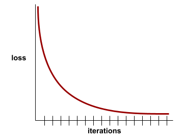
A loss curve plots training loss versus the number of iterations. A loss curve provides the following hints about training:
- A downward slope implies that the model is improving.
- An upward slope implies that the model is getting worse.
- A flat slope implies that the model has reached convergence .
For example, the following somewhat idealized loss curve shows:
- A steep downward slope during the initial iterations, which implies rapid model improvement.
- A gradually flattening (but still downward) slope until close to the end of training, which implies continued model improvement at a somewhat slower pace then during the initial iterations.
- A flat slope towards the end of training, which suggests convergence.
Although training loss is important, see also generalization .
Trivia Question Answering
Datasets to evaluate an LLM's ability to answer trivia questions. Each dataset contains question-answer pairs authored by trivia enthusiasts. Different datasets are grounded by different sources, including:
- Web search (TriviaQA)
- Wikipedia (TriviaQA_wiki)
For more information see TriviaQA: A Large Scale Distantly Supervised Challenge Dataset for Reading Comprehension .
true negative (TN)
An example in which the model correctly predicts the negative class . For example, the model infers that a particular email message is not spam , and that email message really is not spam .
true positive (TP)
An example in which the model correctly predicts the positive class . For example, the model infers that a particular email message is spam, and that email message really is spam.
true positive rate (TPR)
Synonym for recall . That is:
True positive rate is the y-axis in an ROC curve .
Typologically Diverse Question Answering (TyDi QA)
A large dataset for evaluating an LLM's proficiency in answering questions. The dataset contains question and answer pairs in many languages.
For details, see TyDi QA: A Benchmark for Information-Seeking Question Answering in Typologically Diverse Languages .
U
unsupported-claim rate (UCR)
The percentage of claims in a response that aren't grounded . For example, if an LLM's response makes 10 claims but only 1 is grounded, the UCR is 90%.
A high UCR implies that an LLM is hallucinating too frequently.
See also citation precision and citation recall .
ভি
validation loss
A metric representing a model's loss on the validation set during a particular iteration of training.
See also generalization curve .
variable importances
A set of scores that indicates the relative importance of each feature to the model.
For example, consider a decision tree that estimates house prices. Suppose this decision tree uses three features: size, age, and style. If a set of variable importances for the three features are calculated to be {size=5.8, age=2.5, style=4.7}, then size is more important to the decision tree than age or style.
Different variable importance metrics exist, which can inform ML experts about different aspects of models.
ডাব্লিউ
Wasserstein loss
One of the loss functions commonly used in generative adversarial networks , based on the earth mover's distance between the distribution of generated data and real data.
WiC
Abbreviation for Words in Context .
WikiLingua (wiki_lingua)
A dataset for evaluating an LLM's ability to summarize short articles. WikiHow , an encyclopedia of articles explaining how to do various tasks, is the human-authored source for both the articles and the summaries. Each entry in the dataset consists of:
- An article, which is created by appending each step of the prose (paragraph) version of the numbered list, minus the opening sentence of each step.
- A summary of that article, consisting of the opening sentence of each step in the numbered list.
For details, see WikiLingua: A New Benchmark Dataset for Cross-Lingual Abstractive Summarization .
Winograd Schema Challenge (WSC)
A format (or dataset conforming to that format) for evaluating an LLM's ability to determine the noun phrase that a pronoun refers to.
Each entry in a Winograd Schema Challenge consists of:
- A short passage, which contains a target pronoun
- A target pronoun
- Candidate noun phrases, followed by the correct answer (a Boolean). If the target pronoun refers to this candidate, the answer is True. If the target pronoun does not refer to this candidate, the answer is False.
উদাহরণস্বরূপ:
- Passage : Mark told Pete many lies about himself, which Pete included in his book. He should have been more truthful.
- Target pronoun : He
- Candidate noun phrases :
- Mark: True, because the target pronoun refers to Mark
- Pete: False, because the target pronoun doesn't refer to Peter
The Winograd Schema Challenge is a component of the SuperGLUE ensemble.
Words in Context (WiC)
A dataset for evaluating how well an LLM uses context to understand words that have multiple meanings. Each entry in the dataset contains:
- Two sentences, each containing the target word
- The target word
- The correct answer (a Boolean), where:
- True means the target word has the same meaning in the two sentences
- False means the target word has a different meaning in the two sentences
উদাহরণস্বরূপ:
- Two sentences:
- There's a lot of trash on the bed of the river.
- I keep a glass of water next to my bed when I sleep.
- The target word: bed
- Correct answer : False, because the target word has a different meaning in the two sentences.
For details, see WiC: the Word-in-Context Dataset for Evaluating Context-Sensitive Meaning Representations .
Words in Context is a component of the SuperGLUE ensemble.
WSC
Abbreviation for Winograd Schema Challenge .
এক্স
XL-Sum (xlsum)
A dataset for evaluating an LLM's proficiency in summarizing text. XL-Sum provides entries in many languages. Each entry in the dataset contains:
- An article, taken from the British Broadcasting Company (BBC).
- A summary of the article, written by the article's author. Note that that summary can contain words or phrases not present in the article.
For details, see XL-Sum: Large-Scale Multilingual Abstractive Summarization for 44 Languages .