التصنيف: ROC وAUC

قدّم القسم السابق مجموعة من مقاييس النماذج، تم احتسابها جميعًا عند قيمة حدّ تصنيف واحد. ولكن إذا كنت تريد تقييم جودة النموذج على جميع الحدود الممكنة، ستحتاج إلى أدوات مختلفة.

منحنى الخصائص التشغيلية للمستقبِل (ROC)

منحنى ROC هو تمثيل مرئي لأداء النموذج في جميع العتبات. إنّ النسخة الطويلة من الاسم، وهي خاصية تشغيل جهاز الاستقبال، هي بقايا من تكنولوجيا رصد الرادار في الحرب العالمية الثانية.

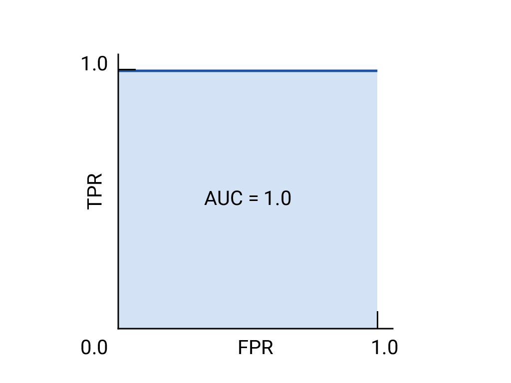
يتم رسم منحنى ROC من خلال احتساب معدّل الموجب الصحيح (TPR) ومعدّل الموجب الخاطئ (FPR) عند كل حدّ ممكن (في الممارسة العملية، عند فواصل زمنية محدّدة)، ثمّ رسم معدّل الموجب الصحيح على معدّل الموجب الخاطئ. يمكن تمثيل نموذج مثالي، الذي يحقّق نسبة إيجابية حقيقية تبلغ 1.0 ونسبة خطأ إيجابية تبلغ 0.0 عند حدّ معيّن، بنقطة عند (0, 1) في حال تجاهل جميع الحدود الأخرى، أو بما يلي:

الشكل 1. منحنى خاصية تشغيل جهاز الاستقبال ومساحة تحت منحنى الأداء لنموذج مثالي افتراضي

المساحة تحت المنحنى (AUC)

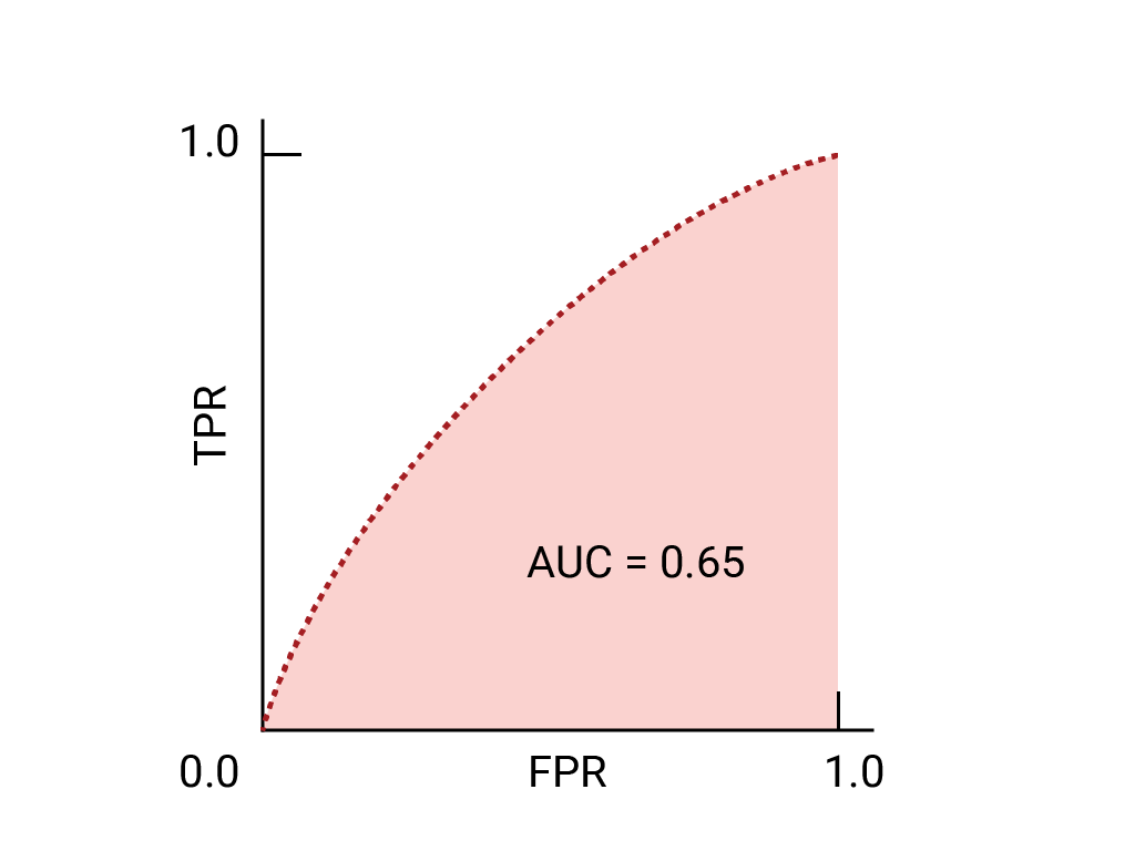
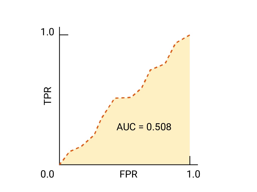
تمثل المنطقة تحت منحنى ROC (AUC) احتمالية أن يصنّف النموذج المثال الموجب على أنّه أعلى من المثال السلبي، إذا تم تقديم مثال موجب ومثال سلبي تم اختيارهما عشوائيًا.

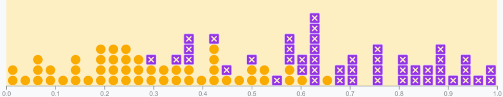
النموذج المثالي أعلاه الذي يحتوي على مربّع أضلاعه بطول 1 له مساحة تحت المنحنى (AUC) تبلغ 1.0. وهذا يعني أنّ هناك احتمالية بنسبة% 100 أن يصنّف النموذج بشكل صحيح مثالاً إيجابيًا تم اختياره عشوائيًا أعلى من مثال سلبي تم اختياره عشوائيًا. بعبارة أخرى، عند الاطّلاع على انتشار نقاط data أدناه، يقدّم مقياس AUC احتمالية أن يضع النموذج مربعًا تم اختياره عشوائيًا على يسار دائرة تم اختيارها عشوائيًا، بغض النظر عن مكان ضبط الحدّ الأدنى.

بعبارة أكثر تحديدًا، يحدِّد نظام تصنيف الرسائل غير المرغوب فيها الذي يمتلك AUC ‏1.0 دائمًا احتمالية أعلى بأن تكون رسالة إلكترونية عشوائية غير مرغوب فيها غير مرغوب فيها مقارنةً برسالة إلكترونية عشوائية صالحة. يعتمد التصنيف الفعلي لكل بريد إلكتروني على الحدّ الأدنى الذي تختاره.

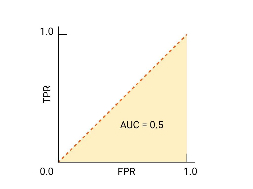
بالنسبة إلى المصنّف الثنائي، يُعدّ النموذج الذي يحقّق أداءً مماثلاً تمامًا للتوقّعات العشوائية أو رمي العملات المعدنية هو نموذج ROC الذي يمثّل خطًا قطريًا من (0,0) إلى (1,1). تكون دالة AUC هي 0.5، ما يمثّل احتمالية بنسبة% 50 لترتيب مثال إيجابي و سلبي عشوائي بشكل صحيح.

في مثال معرّف الرسائل غير المرغوب فيها، يحدِّد معرّف الرسائل غير المرغوب فيها الذي يبلغ AUC‏ 0.5 احتمالية أعلى بأن تكون رسائل إلكترونية عشوائية غير مرغوب فيها مقارنةً برسائل إلكترونية عشوائية مرغوب فيها في نصف الوقت فقط.

الشكل 2. منحنى ROC وAUC للتخمينات العشوائية تمامًا

(اختياري ومتقدّم) منحنى الدقة والاستذكار

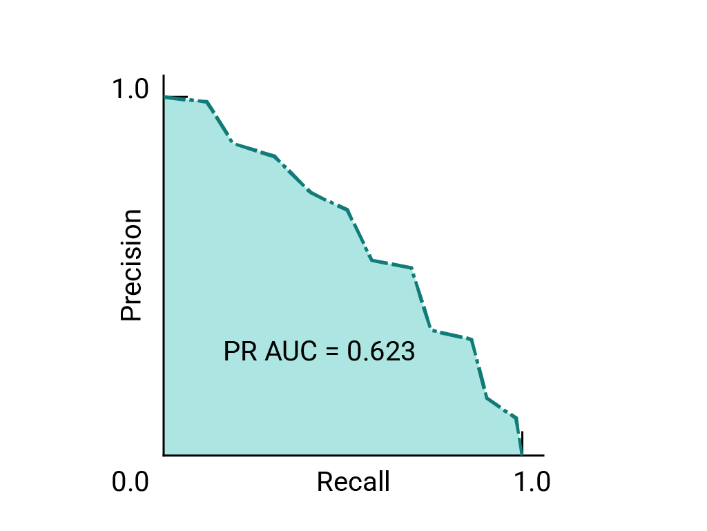
يعمل مقياسا AUC وROC بشكل جيد لمقارنة النماذج عندما تكون مجموعة البيانات متوازنة تقريبًا بين الفئات. عندما تكون مجموعة البيانات غير متوازنة، قد تقدّم منحنيات الدقة-الاسترجاع (PRC) والمساحة تحت هذه المنحنيات تمثيلاً مرئيًا مقارنةً أفضل لأداء النموذج. يتم إنشاء منحنيات الدقة والتذكر من خلال رسم الدقة على المحور y وتذكر على المحور x على مستوى كل الحدود الدنيا.

AUC وROC لاختيار النموذج والحدّ الأدنى

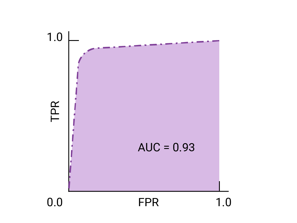
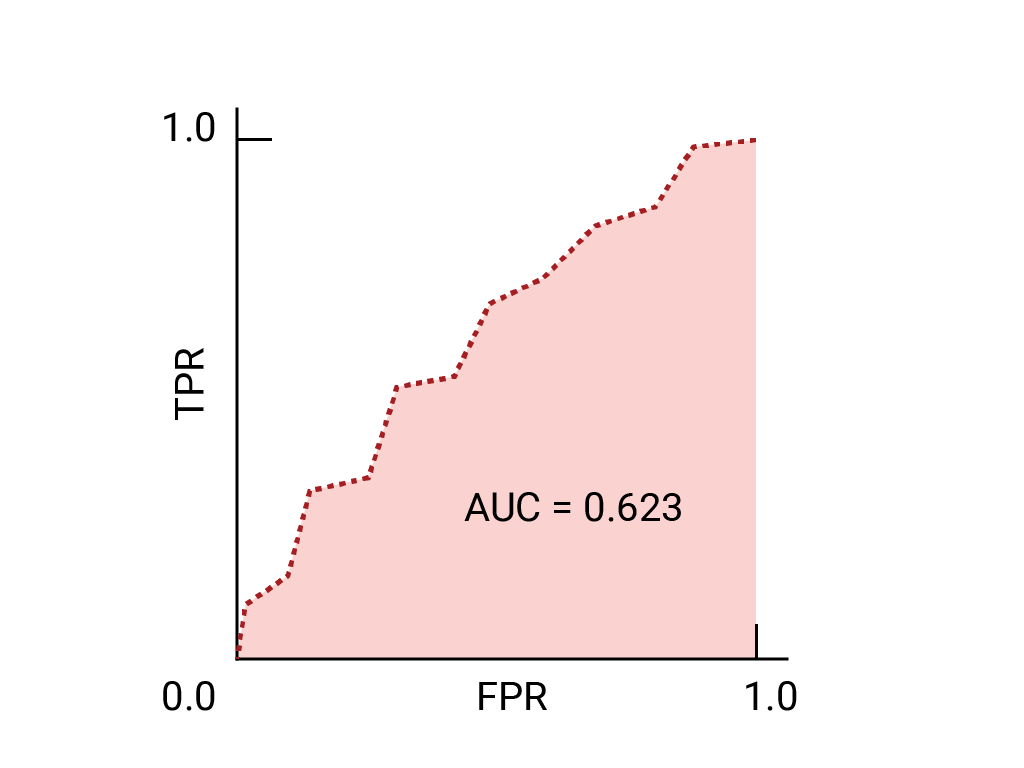
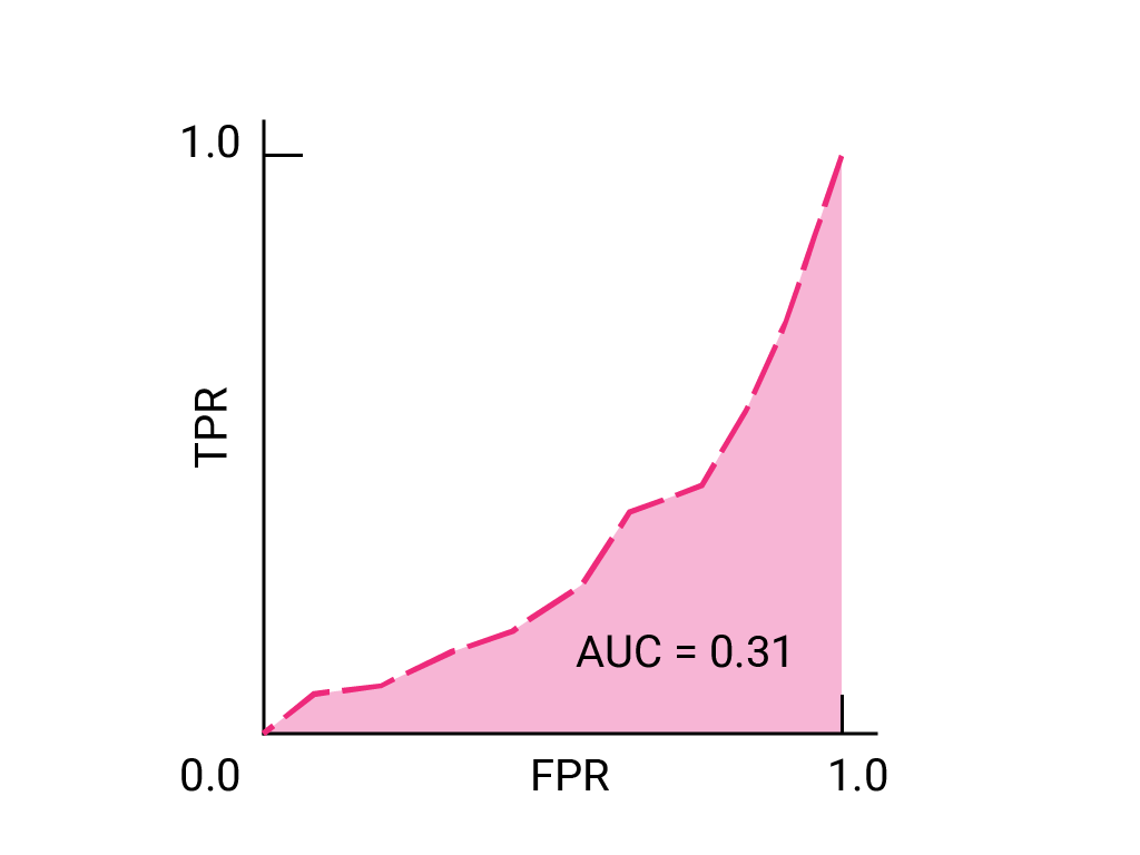
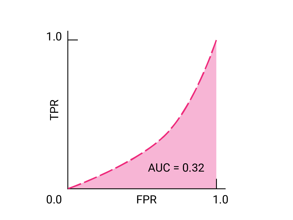
يُعدّ مقياس AUC مقياسًا مفيدًا لمقارنة أداء نموذجَين مختلفَين، ما دامت مجموعة البيانات متوازنة تقريبًا. بشكل عام، يكون النموذج الذي يضم مساحة أكبر تحت المنحنى هو الأفضل.

الشكل 3. منحنى ROC ومساحة تحت منحنى ROC لنموذجَين افتراضيَين يمثّل المنحنى على اليسار، الذي يضمّ مؤشرًا أكبر لمنطقة تحت منحنى ROC، أفضل هذين النموذجَين.

تمثّل النقاط على منحنى ROC الأقرب إلى (0,1) نطاقًا من الحدود الدنيا الأفضل أداءً للنموذج المحدّد. كما هو موضّح في أقسام الحدود الدنيا، مصفوفة الالتباس و اختيار المقياس والمفاضلات ، يعتمد الحدّ الأدنى الذي تختاره على المقياس الأكثر أهمية لحالة الاستخدام المحدّدة. فكِّر في النقاط "أ" و"ب" و"ج" في الرسم البياني التالي، والتي تمثّل كلٌّ منها حدًا:

الشكل 4. ثلاث نقاط مصنّفة تمثّل الحدود الدنيا

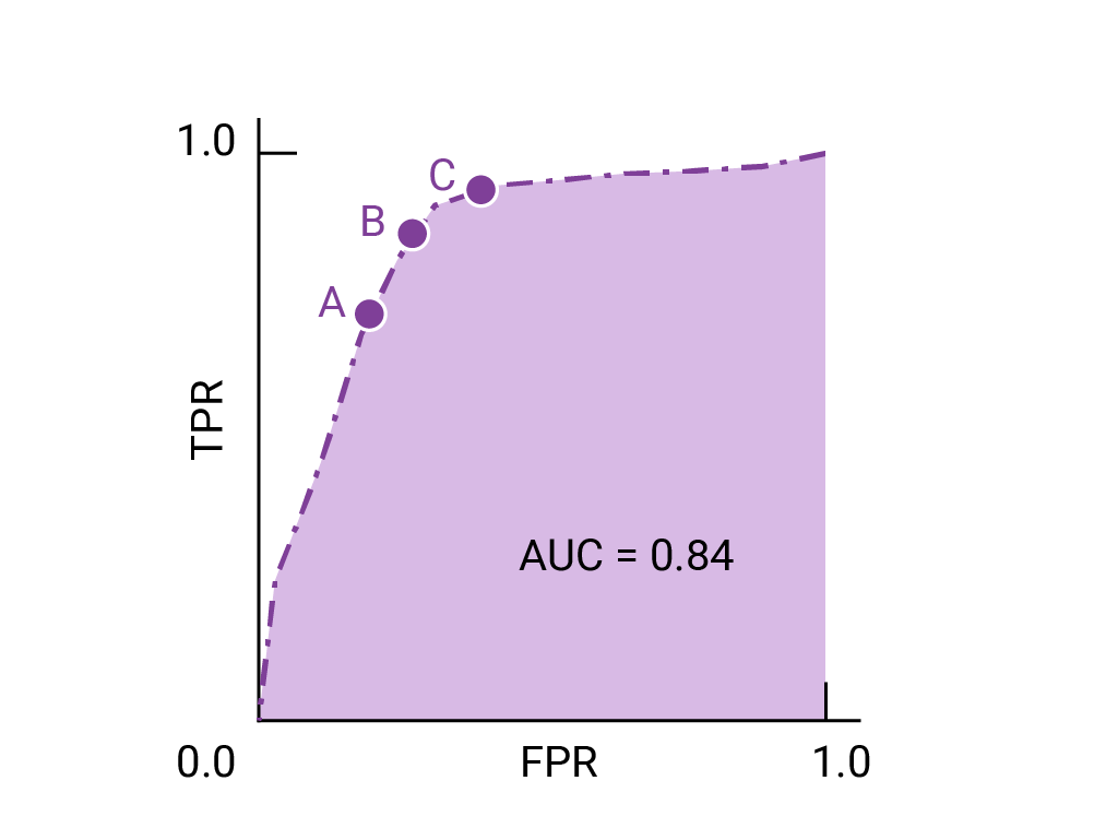
إذا كانت النتائج الإيجابية الخاطئة (الإشعارات الخاطئة) باهظة التكلفة، قد يكون من المنطقي اختيار حدّ يقدّم معدّل خطأ إيجابي أقلّ، مثل المعدّل في النقطة "أ"، حتى إذا تم خفض TPR. في المقابل، إذا كانت النتائج الموجبة الخاطئة منخفضة التكلفة والنتائج السالبة الخاطئة (النتائج الموجبة الصائبة الفائتة) مرتفعة التكلفة، قد يكون الحدّ الأدنى للنقطة "ج"، الذي يحقّق الحد الأقصى لنسبة النتائج الموجبة الصائبة، هو الخيار المفضّل. إذا كانت التكاليف متكافئة تقريبًا، قد تقدّم النقطة ب أفضل توازن بين معدّل الإحالات الناجحة النسبي ومعدّل الإحالات الناجحة الإجمالي.

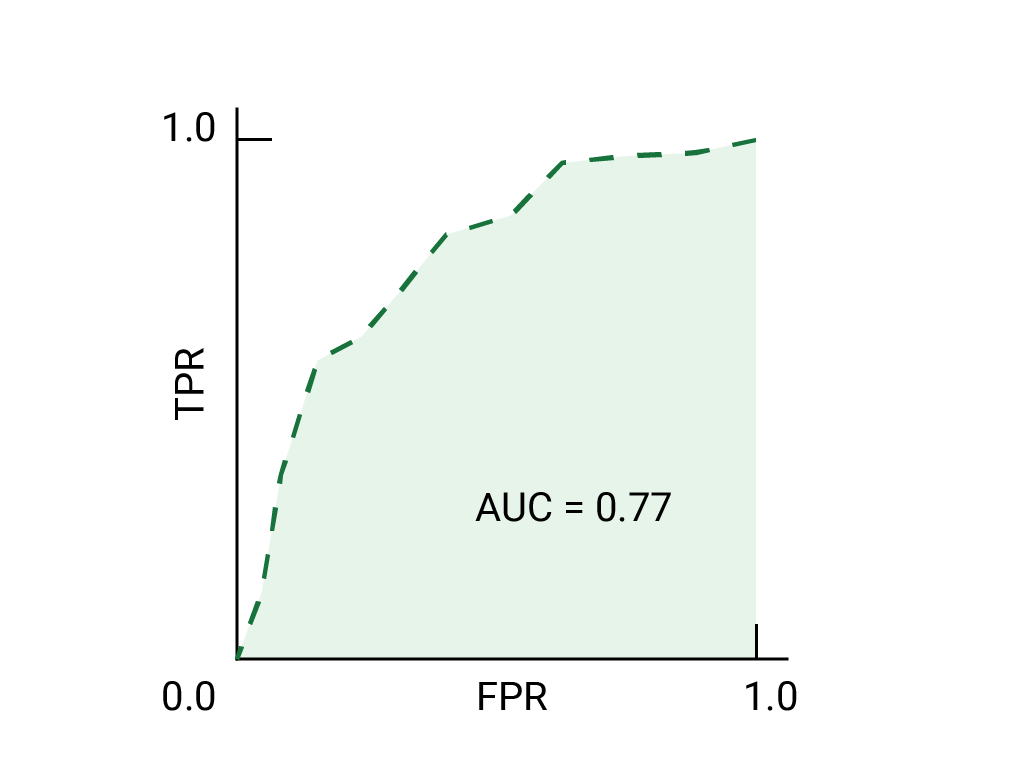
في ما يلي منحنى ROC للبيانات التي سبق أن رأيناها:

تمرين: التحقّق من فهمك

في الممارسة العملية، تكون منحنيات ROC أقل انتظامًا بكثير من الرسومات التوضيحية الواردة أعلاه. أيٌّ من النماذج التالية، التي يمثّلها منحنى ROC ومعامل AUC، يحقّق أفضل أداء؟

يحقّق هذا النموذج أعلى قيمة لمقياس AUC، ما يتوافق مع أفضل أداء.

أيّ من النماذج التالية يحقّق أداءً أسوأ من الصدفة؟

يُظهر هذا النموذج قيمة AUC أقل من 0.5، ما يعني أنّ أدائه أسوأ من الصدفة.

يحقّق هذا النموذج أداءً أفضل قليلاً من الصدفة.

يحقّق هذا النموذج الأداء نفسه الذي يحقّقه الاختيار العشوائي.

هذا هو تصنيف مثالي افتراضي.

(اختياري ومتقدّم) سؤال إضافي

أيّ من التغييرات التالية يمكن إجراؤها على نموذج "الأداء أسوأ من الصدفة" في السؤال السابق لتحسين أدائه؟

اقلب التوقعات، بحيث تصبح التوقعات التي تبلغ 1 0، والتوقعات التي تبلغ 0 1.

إذا كان المصنّف الثنائي يضع الأمثلة في الفئات الخاطئة بشكل موثوق أكثر من الصدفة، يؤدي تبديل تصنيف الفئة على الفور إلى تحسين توقّعاته عن الصدفة بدون الحاجة إلى إعادة تدريب النموذج.

اطلب من النموذج أن يتوقّع دائمًا الفئة السلبية.

وقد يؤدي ذلك إلى تحسين الأداء أو لا يؤدي إلى ذلك. بالإضافة إلى ذلك، كما هو موضح في قسم الدقة، هذا النموذج ليس مفيدًا.

اطلب منه توقّع الفئة الموجبة دائمًا.

وقد يؤدي ذلك إلى تحسين الأداء أو لا يؤدي إلى ذلك. بالإضافة إلى ذلك، كما هو موضح في قسم الدقة، ليس هذا النموذج مفيدًا.

تخيل موقفًا يكون فيه من الأفضل السماح لبعض الرسائل غير المرغوب فيها بالوصول إلى البريد الوارد بدلاً من إرسال رسالة إلكترونية مهمة للنشاط التجاري إلى مجلد الرسائل غير المرغوب فيها. لقد دربت أحد أدوات تصنيف الرسائل غير المرغوب فيها لهذا الموقف حيث تكون الفئة الموجبة هي الرسائل غير المرغوب فيها والفئة السالبة هي الرسائل غير غير المرغوب فيها. أيّ من النقاط التالية على منحنى ROC لفلترة البيانات هو الأفضل؟

النقطة "أ"

في حالة الاستخدام هذه، من الأفضل تقليل النتائج الموجبة الخاطئة، حتى إذا انخفضت أيضًا النتائج الموجبة الصائبة.

النقطة ب

يوازن هذا الحدّ النتائج الموجبة الصائبة والخاطئة.

النقطة ج

ويؤدي هذا الحدّ إلى زيادة الإيجابيات الحقيقية إلى أقصى حدّ (الإبلاغ عن المزيد من الرسائل غير المرغوب فيها) على حساب زيادة الإيجابيات الخاطئة (الإبلاغ عن المزيد من الرسائل الإلكترونية المشروعة على أنّها غير مرغوب فيها).

المصطلحات الرئيسية:

• المساحة تحت منحنى ROC (AUC)
• منحنى ROC

مركز المساعدة