
1. 시작하기 전에
이 Codelab에서는 컨볼루션을 사용하여 말과 사람의 이미지를 분류합니다. 이 실습에서는 TensorFlow를 사용하여 말과 사람의 이미지를 인식하고 분류하는 교육을 받은 CNN을 만듭니다.
기본 요건
이전에 TensorFlow로 컨볼루션을 빌드한 적이 없는 경우 컨볼루션 및 풀링을 도입한 컨볼루션 빌드 및 풀링 Codelab을 완료하고, 컴퓨터 비전을 향상하기 위해 컨볼루셔널 신경망 (CNN)을 빌드함으로써 이미지를 더 효율적으로 인식하는 방법을 알아보세요.
학습할 내용
- 피사체가 명확하지 않은 이미지에서 특징을 인식하도록 컴퓨터를 학습시키는 방법
빌드할 항목
- 말 사진과 사람의 사진을 구별할 수 있는 컨볼루셔널 신경망
필요한 항목
Colab에서 실행되는 나머지 Codelab용 코드를 찾을 수 있습니다.
또한 TensorFlow와 이전 Codelab에 설치한 라이브러리도 필요합니다.
2. 시작하기: 데이터 가져오기
말 또는 인간이 포함된 이미지가 빌드되면 말이나 인간이 포함되어 있는지 알 수 있는 말 또는 인간 분류기를 만들어 네트워크가 어떤 특징이 있는지 판단하도록 모델을 학습시키는지 확인할 수 있습니다. 학습하기 전에 먼저 데이터를 일부 처리해야 합니다.
먼저 다음과 같이 데이터를 다운로드합니다.
!wget --no-check-certificate https://storage.googleapis.com/laurencemoroney-blog.appspot.com/horse-or-human.zip -O /tmp/horse-or-human.zip
다음 Python 코드는 OS 라이브러리를 사용하여 운영체제 라이브러리를 사용합니다. 이를 통해 파일 시스템 및 zip 파일 라이브러리에 액세스할 수 있으므로 데이터의 압축을 풀 수 있습니다.
import os
import zipfile

local_zip = '/tmp/horse-or-human.zip'
zip_ref = zipfile.ZipFile(local_zip, 'r')
zip_ref.extractall('/tmp/horse-or-human')
zip_ref.close()
ZIP 파일의 콘텐츠는 말과 사람의 하위 디렉터리가 포함된 기본 디렉터리 /tmp/horse-or-human에 추출됩니다.
간단히 말해 학습 세트는 말이 어떤 모습인지, 그리고 인간이 어떤 모습인지를 신경망 모델에 알려주는 데 사용되는 데이터입니다.
3. ImageGenerator를 사용하여 데이터에 라벨 지정 및 준비하기
이미지에 말이나 사람의 라벨을 명시적으로 지정하지 않습니다.
나중에 ImageDataGenerator이 사용 중인 것을 볼 수 있습니다. 하위 디렉터리의 이미지를 읽고 해당 하위 디렉터리의 이름으로부터 자동으로 라벨을 지정합니다. 예를 들어 말 디렉터리와 인간 디렉터리가 포함된 학습 디렉터리가 있습니다. ImageDataGenerator가 이미지에 적절하게 라벨을 지정하여 코딩 단계를 줄입니다.
이러한 각 디렉터리를 정의합니다.
# Directory with our training horse pictures
train_horse_dir = os.path.join('/tmp/horse-or-human/horses')

# Directory with our training human pictures
train_human_dir = os.path.join('/tmp/horse-or-human/humans')
이제 말과 인간 교육 디렉터리에서 파일 이름이 어떻게 표시되는지 확인합니다.
train_horse_names = os.listdir(train_horse_dir)
print(train_horse_names[:10])
train_human_names = os.listdir(train_human_dir)
print(train_human_names[:10])
디렉터리에서 말과 사람의 이미지의 총 개수를 확인합니다.
print('total training horse images:', len(os.listdir(train_horse_dir)))
print('total training human images:', len(os.listdir(train_human_dir)))
4. 데이터 살펴보기
사진을 몇 장 보고 어떤 모습인지 더 잘 파악할 수 있습니다.
먼저 matplot 매개변수를 구성합니다.
%matplotlib inline

import matplotlib.pyplot as plt
import matplotlib.image as mpimg

# Parameters for our graph; we'll output images in a 4x4 configuration
nrows = 4
ncols = 4

# Index for iterating over images
pic_index = 0
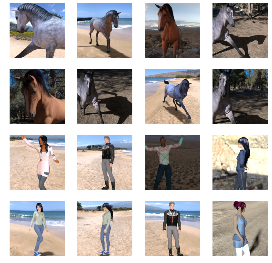
이제 8개의 말 사진과 8개의 인간 사진을 일괄적으로 표시합니다. 셀을 다시 실행하여 매번 새로운 배치를 볼 수 있습니다.
# Set up matplotlib fig, and size it to fit 4x4 pics
fig = plt.gcf()
fig.set_size_inches(ncols * 4, nrows * 4)

pic_index += 8
next_horse_pix = [os.path.join(train_horse_dir, fname)
                for fname in train_horse_names[pic_index-8:pic_index]]
next_human_pix = [os.path.join(train_human_dir, fname)
                for fname in train_human_names[pic_index-8:pic_index]]

for i, img_path in enumerate(next_horse_pix+next_human_pix):
  # Set up subplot; subplot indices start at 1
  sp = plt.subplot(nrows, ncols, i + 1)
  sp.axis('Off') # Don't show axes (or gridlines)

  img = mpimg.imread(img_path)
  plt.imshow(img)

plt.show()
다음은 다양한 포즈와 방향의 말과 인간을 보여 주는 몇 가지 이미지의 예입니다.
5. 모델 정의
모델 정의를 시작합니다.
TensorFlow를 가져와 시작합니다.
import tensorflow as tf
그런 다음 컨볼루셔널 레이어를 추가하고 최종 결과를 평면화하여 밀집 레이어에 데이터를 공급합니다. 마지막으로 밀집된 계층을 추가합니다.
두 가지 분류 문제(바이너리 분류 문제)에 직면했을 때 네트워크의 출력이 0과 1 사이의 스칼라가 되어 현재 이미지가 클래스 0이 아닌 클래스 1이 될 확률을 인코딩하도록 시그모이드 활성화가 됩니다.
model = tf.keras.models.Sequential([
    # Note the input shape is the desired size of the image 300x300 with 3 bytes color
    # This is the first convolution
    tf.keras.layers.Conv2D(16, (3,3), activation='relu', input_shape=(300, 300, 3)),
    tf.keras.layers.MaxPooling2D(2, 2),
    # The second convolution
    tf.keras.layers.Conv2D(32, (3,3), activation='relu'),
    tf.keras.layers.MaxPooling2D(2,2),
    # The third convolution
    tf.keras.layers.Conv2D(64, (3,3), activation='relu'),
    tf.keras.layers.MaxPooling2D(2,2),
    # The fourth convolution
    tf.keras.layers.Conv2D(64, (3,3), activation='relu'),
    tf.keras.layers.MaxPooling2D(2,2),
    # The fifth convolution
    tf.keras.layers.Conv2D(64, (3,3), activation='relu'),
    tf.keras.layers.MaxPooling2D(2,2),
    # Flatten the results to feed into a DNN
    tf.keras.layers.Flatten(),
    # 512 neuron hidden layer
    tf.keras.layers.Dense(512, activation='relu'),
    # Only 1 output neuron. It will contain a value from 0-1 where 0 for 1 class ('horses') and 1 for the other ('humans')
    tf.keras.layers.Dense(1, activation='sigmoid')
])
model.summary() 메서드 호출은 네트워크의 요약을 출력합니다.
model.summary()
여기에서 결과를 확인할 수 있습니다.
Layer (type)                 Output Shape              Param #
=================================================================
conv2d (Conv2D)              (None, 298, 298, 16)      448
_________________________________________________________________
max_pooling2d (MaxPooling2D) (None, 149, 149, 16)      0
_________________________________________________________________
conv2d_1 (Conv2D)            (None, 147, 147, 32)      4640
_________________________________________________________________
max_pooling2d_1 (MaxPooling2 (None, 73, 73, 32)        0
_________________________________________________________________
conv2d_2 (Conv2D)            (None, 71, 71, 64)        18496
_________________________________________________________________
max_pooling2d_2 (MaxPooling2 (None, 35, 35, 64)        0
_________________________________________________________________
conv2d_3 (Conv2D)            (None, 33, 33, 64)        36928
_________________________________________________________________
max_pooling2d_3 (MaxPooling2 (None, 16, 16, 64)        0
_________________________________________________________________
conv2d_4 (Conv2D)            (None, 14, 14, 64)        36928
_________________________________________________________________
max_pooling2d_4 (MaxPooling2 (None, 7, 7, 64)          0
_________________________________________________________________
flatten (Flatten)            (None, 3136)              0
_________________________________________________________________
dense (Dense)                (None, 512)               1606144
_________________________________________________________________
dense_1 (Dense)              (None, 1)                 513
=================================================================
Total params: 1,704,097
Trainable params: 1,704,097
Non-trainable params: 0
출력 셰이프 열은 연속된 각 레이어에서 특성 맵의 크기가 어떻게 발전하는지 보여줍니다. 컨볼루션 레이어는 패딩으로 인해 특성 맵의 크기를 조금 줄입니다. 각 풀링 레이어는 크기를 절반으로 나눕니다.
6. 모델 컴파일
다음으로 모델 학습 사양을 구성합니다. 이진 분류 문제이며 최종 활성화는 시그모이드이므로 binary_crossentropy 손실로 모델을 학습시킵니다. 손실 측정항목에 대한 복습은 ML로 다운그레이드하기를 참고하세요. 학습률이 0.001인 rmsprop 최적화 도구를 사용합니다. 학습 중에 분류 정확성을 모니터링합니다.
from tensorflow.keras.optimizers import RMSprop

model.compile(loss='binary_crossentropy',
              optimizer=RMSprop(lr=0.001),
              metrics=['acc'])
7. 생성기에서 모델 학습
소스 생성기에서 사진을 읽고 float32 텐서로 변환한 후 라벨을 사용하여 데이터 생성기를 네트워크에 공급할 수 있습니다.
학습용 이미지 및 학습용 이미지의 생성기가 하나씩 있습니다. Generator는 300x300 크기 및 해당 라벨 (바이너리)의 이미지 배치를 생성합니다.
아시다시피 일반적으로 신경망로 들어오는 데이터는 네트워크에서 더 쉽게 처리할 수 있도록 어떤 방식으로 정규화되어야 합니다. CNN에 원시 픽셀을 공급하는 것은 드문 일입니다. 이 경우에는 픽셀 값을 [0, 1] 범위에 포함하도록 정규화하여 이미지를 사전 처리합니다 (원래 모든 값은 [0, 255] 범위에 있음).
Keras에서는 rescale 매개변수를 사용하여 keras.preprocessing.image.ImageDataGenerator 클래스를 통해 실행할 수 있습니다. 이 ImageDataGenerator 클래스를 사용하면 .flow(데이터, 라벨) 또는 .flow_from_directory(directory)를 통해 증강된 이미지 배치 및 해당 라벨의 생성기를 인스턴스화할 수 있습니다. 그런 다음, 이러한 생성기를 데이터 생성기를 입력으로 허용하는 Keras 모델 메서드(fit_generator, evaluate_generator, predict_generator)와 함께 사용할 수 있습니다.
from tensorflow.keras.preprocessing.image import ImageDataGenerator

# All images will be rescaled by 1./255
train_datagen = ImageDataGenerator(rescale=1./255)

# Flow training images in batches of 128 using train_datagen generator
train_generator = train_datagen.flow_from_directory(
        '/tmp/horse-or-human/',  # This is the source directory for training images
        target_size=(300, 300),  # All images will be resized to 150x150
        batch_size=128,
        # Since we use binary_crossentropy loss, we need binary labels
        class_mode='binary')
8. 교육하기
15세대 동안 학습하세요. 실행하는 데 몇 분 정도 걸릴 수 있습니다.
history = model.fit(
      train_generator,
      steps_per_epoch=8,
      epochs=15,
      verbose=1)
에포크별 값을 확인합니다.
손실 및 정확성은 학습 진행 상황을 잘 나타냅니다. 학습 데이터를 분류한 다음 알려진 라벨을 기준으로 측정하여 결과를 계산하는 과정입니다. 정확성은 정확한 추측의 일부입니다.
Epoch 1/15
9/9 [==============================] - 9s 1s/step - loss: 0.8662 - acc: 0.5151
Epoch 2/15
9/9 [==============================] - 8s 927ms/step - loss: 0.7212 - acc: 0.5969
Epoch 3/15
9/9 [==============================] - 8s 921ms/step - loss: 0.6612 - acc: 0.6592
Epoch 4/15
9/9 [==============================] - 8s 925ms/step - loss: 0.3135 - acc: 0.8481
Epoch 5/15
9/9 [==============================] - 8s 919ms/step - loss: 0.4640 - acc: 0.8530
Epoch 6/15
9/9 [==============================] - 8s 896ms/step - loss: 0.2306 - acc: 0.9231
Epoch 7/15
9/9 [==============================] - 8s 915ms/step - loss: 0.1464 - acc: 0.9396
Epoch 8/15
9/9 [==============================] - 8s 935ms/step - loss: 0.2663 - acc: 0.8919
Epoch 9/15
9/9 [==============================] - 8s 883ms/step - loss: 0.0772 - acc: 0.9698
Epoch 10/15
9/9 [==============================] - 9s 951ms/step - loss: 0.0403 - acc: 0.9805
Epoch 11/15
9/9 [==============================] - 8s 891ms/step - loss: 0.2618 - acc: 0.9075
Epoch 12/15
9/9 [==============================] - 8s 902ms/step - loss: 0.0434 - acc: 0.9873
Epoch 13/15
9/9 [==============================] - 8s 904ms/step - loss: 0.0187 - acc: 0.9932
Epoch 14/15
9/9 [==============================] - 9s 951ms/step - loss: 0.0974 - acc: 0.9649
Epoch 15/15
9/9 [==============================] - 8s 877ms/step - loss: 0.2859 - acc: 0.9338
9. 모델 테스트
이제 모델을 사용하여 실제로 예측을 실행합니다. 코드를 사용하면 파일 시스템에서 하나 이상의 파일을 선택할 수 있습니다. 그런 다음 객체를 업로드하고 모델을 통해 실행함으로써 객체가 말인지 아니면 인간인지 표시합니다.
인터넷에서 파일 시스템으로 이미지를 다운로드하여 사용해 볼 수 있습니다. 학습 정확도가 99%를 초과하더라도 네트워크에 많은 실수가 있을 수 있습니다.
이는 과적합이라는 문제로 인해 신경망이 매우 제한된 데이터로 학습되었음을 의미합니다 (각 클래스의 이미지 약 500개만 있음). 따라서 학습 세트에 있는 것과 유사한 이미지를 인식하는 데는 매우 적합하지만 학습 세트에 없는 이미지에서는 상당히 실패할 수 있습니다.
더 많은 데이터를 학습할수록 최종 네트워크가 더 좋아진다는 것을 보여주는 데이터 포인트입니다.
이미지 증강이라는 것을 포함하여 제한된 데이터라도 학습을 개선할 수 있는 여러 가지 방법이 있지만 이 Codelab에서 다루지는 않습니다.
import numpy as np
from google.colab import files
from keras.preprocessing import image

uploaded = files.upload()

for fn in uploaded.keys():

  # predicting images
  path = '/content/' + fn
  img = image.load_img(path, target_size=(300, 300))
  x = image.img_to_array(img)
  x = np.expand_dims(x, axis=0)

  images = np.vstack([x])
  classes = model.predict(images, batch_size=10)
  print(classes[0])
  if classes[0]>0.5:
    print(fn + " is a human")
  else:
    print(fn + " is a horse")
예를 들어 이 이미지로 테스트한다고 가정해 보겠습니다.

Colab에서 생성되는 데이터는 다음과 같습니다.
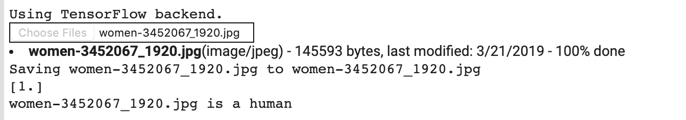
만화책이라 하더라도 올바르게 분류되는 콘텐츠입니다.
다음 이미지도 올바르게 분류됩니다.
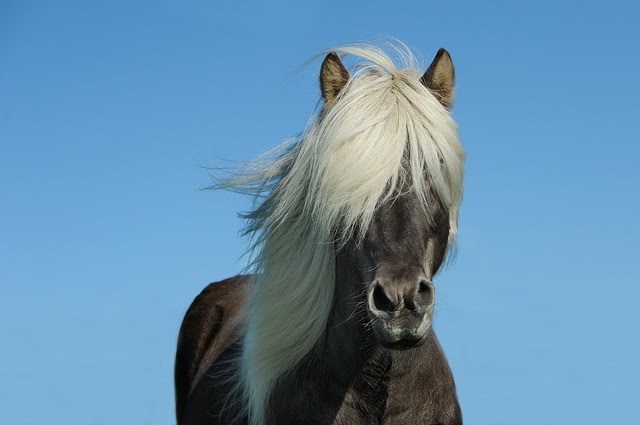
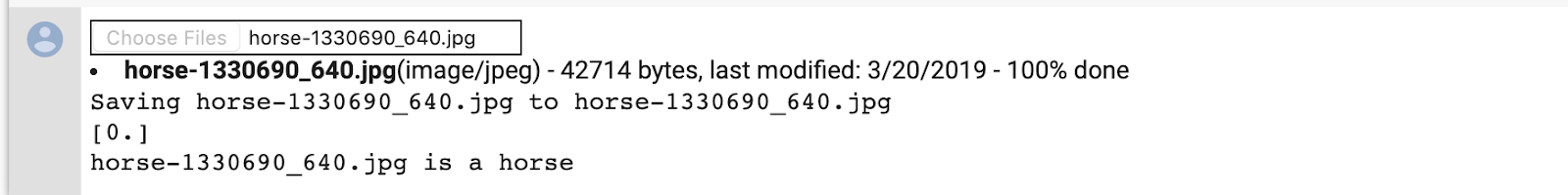
직접 이미지를 사용해 보세요.
10. 중간 표현 시각화
CNN이 학습한 특성의 종류를 알아보려면 CNN을 통과할 때 입력이 어떻게 변환되는지 시각화하는 것이 좋습니다.
학습 세트에서 임의 이미지를 선택한 다음 각 행이 레이어의 출력이고 행의 각 이미지가 해당 출력 특성 맵의 특정 필터인 그림을 생성합니다. 이 셀을 다시 실행하여 다양한 학습 이미지에 대한 중간 표현을 생성합니다.
import numpy as np
import random
from tensorflow.keras.preprocessing.image import img_to_array, load_img

# Let's define a new Model that will take an image as input, and will output
# intermediate representations for all layers in the previous model after
# the first.
successive_outputs = [layer.output for layer in model.layers[1:]]
#visualization_model = Model(img_input, successive_outputs)
visualization_model = tf.keras.models.Model(inputs = model.input, outputs = successive_outputs)
# Let's prepare a random input image from the training set.
horse_img_files = [os.path.join(train_horse_dir, f) for f in train_horse_names]
human_img_files = [os.path.join(train_human_dir, f) for f in train_human_names]
img_path = random.choice(horse_img_files + human_img_files)

img = load_img(img_path, target_size=(300, 300))  # this is a PIL image
x = img_to_array(img)  # Numpy array with shape (150, 150, 3)
x = x.reshape((1,) + x.shape)  # Numpy array with shape (1, 150, 150, 3)

# Rescale by 1/255
x /= 255

# Let's run our image through our network, thus obtaining all
# intermediate representations for this image.
successive_feature_maps = visualization_model.predict(x)

# These are the names of the layers, so can have them as part of our plot
layer_names = [layer.name for layer in model.layers]

# Now let's display our representations
for layer_name, feature_map in zip(layer_names, successive_feature_maps):
  if len(feature_map.shape) == 4:
    # Just do this for the conv / maxpool layers, not the fully-connected layers
    n_features = feature_map.shape[-1]  # number of features in feature map
    # The feature map has shape (1, size, size, n_features)
    size = feature_map.shape[1]
    # We will tile our images in this matrix
    display_grid = np.zeros((size, size * n_features))
    for i in range(n_features):
      # Postprocess the feature to make it visually palatable
      x = feature_map[0, :, :, i]
      x -= x.mean()
      if x.std()>0:
        x /= x.std()
      x *= 64
      x += 128
      x = np.clip(x, 0, 255).astype('uint8')
      # We'll tile each filter into this big horizontal grid
      display_grid[:, i * size : (i + 1) * size] = x
    # Display the grid
    scale = 20. / n_features
    plt.figure(figsize=(scale * n_features, scale))
    plt.title(layer_name)
    plt.grid(False)
    plt.imshow(display_grid, aspect='auto', cmap='viridis')
다음은 결과 예입니다.
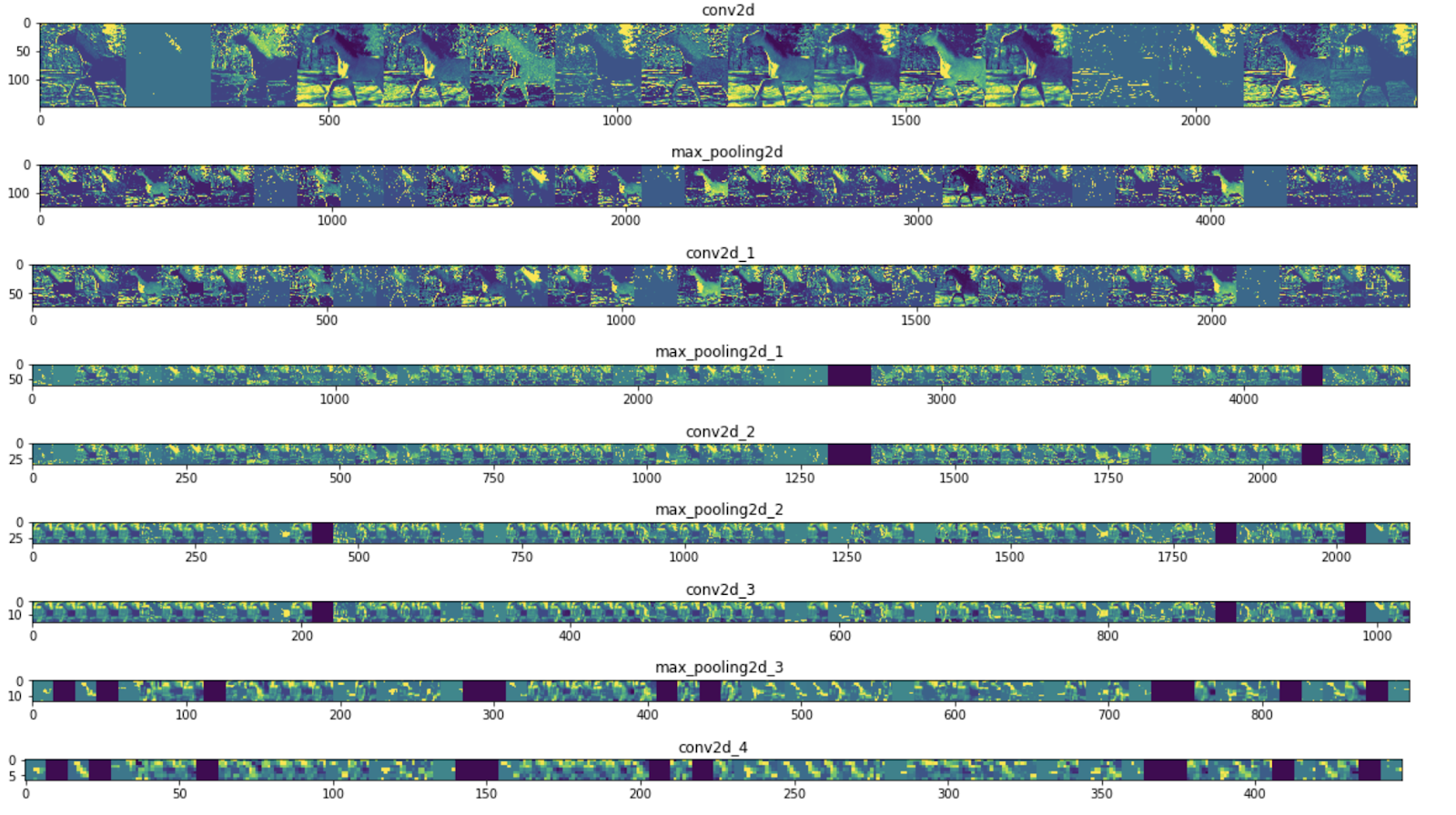
보시다시피 이미지의 원시 픽셀에서 점점 더 추상적이고 간결한 표현으로 이동합니다. 다운스트림 표현은 네트워크에서 주의를 기울여야 하는 부분을 강조하기 시작하고 '활성화'되는 기능이 감소합니다. 대부분 0으로 설정되어 있습니다. 이를 희소성이라고 합니다. 대표성 희소성은 딥 러닝의 핵심 기능입니다.
이러한 표현은 이미지의 원래 픽셀에 대한 정보는 점점 덜 전달하지만 이미지의 클래스에 관한 점점 더 많은 정보를 전달합니다. CNN (일반적으로 딥 네트워크)을 정보 증류 파이프라인이라고 생각하면 됩니다.
11. 축하합니다
CNN을 사용하여 복잡한 이미지를 개선하는 방법을 배웠습니다. 컴퓨터 비전 모델을 더욱 향상시키는 방법을 알아보려면 대규모 데이터 세트를 갖춘 컨볼루셔널 신경망 (CNN)을 사용하여 과적합을 방지하세요.