
1. Introduction
Welcome to the fourth part of the Fundamentals of Apps Script with Google Sheets codelab playlist.
By completing this codelab, you can learn how to format your spreadsheet data in Apps Script, and write functions to create organized spreadsheets full of formatted data fetched from a public API.
What you'll learn
- How to apply various Google Sheets formatting operations in Apps Script.
- How to transform a list of JSON objects and their attributes into an organized sheet of data with Apps Script.
Before you begin
This is the fourth codelab in the Fundamentals of Apps Script with Google Sheets playlist. Before starting this codelab, be sure to complete the previous codelabs:
What you'll need
- An understanding of the basic Apps Script topics explored in the previous codelabs of this playlist.
- Basic familiarity with the Apps Script editor
- Basic familiarity with Google Sheets
- Ability to read Sheets A1 Notation
- Basic familiarity with JavaScript and its
Stringclass
2. Set up
Before you continue, you need a spreadsheet with some data. As before, we've provided a data sheet you can copy for these exercises. Take the following steps:
- Click this link to copy the data sheet and then click Make a copy. The new spreadsheet is placed in your Google Drive folder and named "Copy of Data Formatting".
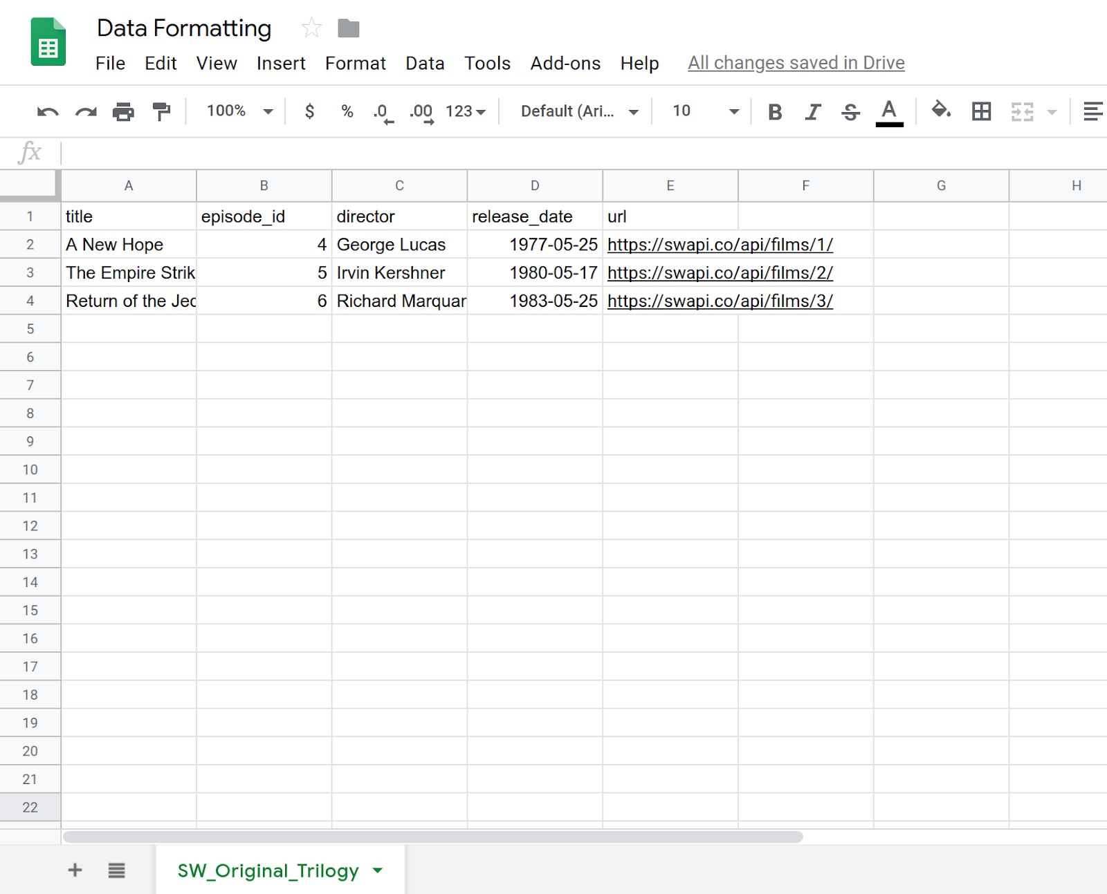
- Click the spreadsheet title and change it from "Copy of Data Formatting" to "Data Formatting". Your sheet should look like this, with some basic information about the first three Star Wars films:
- Select Extensions > Apps Script to open the script editor.
- Click the Apps Script project title and change it from "Untitled project" to "Data Formatting." Click Rename to save the title change.
With this spreadsheet and project, you're ready to start the codelab. Move to the next section to start learning about basic formatting in Apps Script.
3. Create a custom menu
You can apply several basic formatting methods in Apps Script to your Sheets. The following exercises demonstrate a few ways of formatting data. To help control your formatting actions, let's create a custom menu with the items you'll need. The process for creating custom menus was described in the Working with data codelab, but we'll summarize it here again.
Implementation
Let's create a custom menu.
- In the Apps Script editor, replace the code in your script project with the following:
/**
 * A special function that runs when the spreadsheet is opened
 * or reloaded, used to add a custom menu to the spreadsheet.
 */
function onOpen() {
  // Get the spreadsheet's user-interface object.
  var ui = SpreadsheetApp.getUi();

  // Create and add a named menu and its items to the menu bar.
  ui.createMenu('Quick formats')
   .addItem('Format row header', 'formatRowHeader')
   .addItem('Format column header', 'formatColumnHeader')
   .addItem('Format dataset', 'formatDataset')
  .addToUi();
}
- Save your script project.
- In the script editor, select
onOpenfrom the functions list and click Run. This runsonOpen()to rebuild the spreadsheet menu, so you don't have to reload the spreadsheet.
Code review
Let's review this code to understand how it works. In onOpen(), the first line uses the getUi() method to acquire a Ui object representing the user interface of the active spreadsheet this script is bound to.
The next lines create a menu (Quick formats), add menu items (Format row header, Format column header, and Format dataset) to the menu, and then add the menu to the spreadsheet's interface. This is done with the createMenu(caption), addItem(caption, functionName), and addToUi() methods, respectively.
The addItem(caption, functionName) method creates a connection between the menu item label and an Apps Script function that runs when the menu item is selected. For example, selecting the Format row header menu item causes Sheets to attempt to run the formatRowHeader() function (which doesn't exist yet).
Results
In your spreadsheet, click the Quick formats menu to view the new menu items:
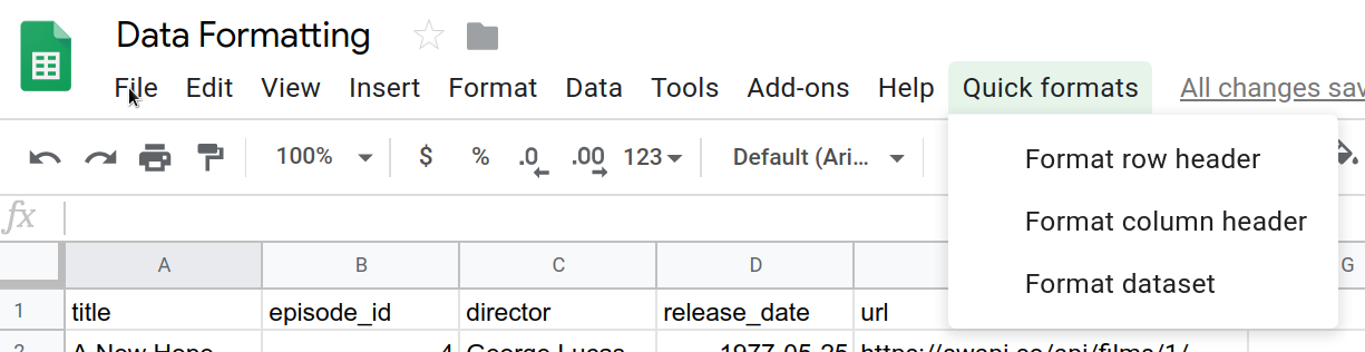
Clicking these items causes an error since you haven't implemented their corresponding functions, so let's do that next.
4. Format a header row
Datasets in spreadsheets often have header rows to identify the data in each column. It's a good idea to format header rows to visually separate them from the rest of the data in the spreadsheet.
In the first codelab, you built a macro for your header and adjusted its code. Here, you'll format a header row from scratch using Apps Script. The header row you'll create will bold the header text, color the background a dark blue-green, color the text white, and add some solid borderlines.
Implementation
To implement the formatting operation, you'll use the same Spreadsheet service methods you've used before, but now you'll also use some of the service's formatting methods. Take the following steps:
- In the Apps Script editor, add the following function to the end of your script project:
/**
 * Formats top row of sheet using our header row style.
 */
function formatRowHeader() {
  // Get the current active sheet and the top row's range.
  var sheet = SpreadsheetApp.getActiveSheet();
  var headerRange = sheet.getRange(1, 1, 1, sheet.getLastColumn());

  // Apply each format to the top row: bold white text,
  // blue-green background, and a solid black border
  // around the cells.
  headerRange
    .setFontWeight('bold')
    .setFontColor('#ffffff')
    .setBackground('#007272')
    .setBorder(
      true, true, true, true, null, null,
      null,
      SpreadsheetApp.BorderStyle.SOLID_MEDIUM);

}
- Save your script project.
Code review
Like many formatting tasks, the Apps Script code to implement it is straightforward. The first two lines use methods you've seen before to get a reference to the current active sheet (sheet) and the top row of the sheet (headerRange). The Sheet.getRange(row, column, numRows, numColumns) method specifies the top row, including only those columns with data in them. The Sheet.getLastColumn() method returns the column index of the last column that contains data in the sheet. In our example, it's column E (url).
The rest of the code simply calls various Range methods to apply formatting choices to all cells in headerRange. To keep the code easy to read, we use method chaining to call each formatting method one after the other:
Range.setFontWeight(fontWeight)is used to set the font weight to bold.Range.setFontColor(color)is used to set the font color to white.Range.setBackground(color)is used to set the background color to a dark blue-green.setBorder(top, left, bottom, right, vertical, horizontal, color, style)puts a solid black border around the range's cells.
The last method has several parameters, so let's review what each is doing. The first four parameters here (all set to true) tell Apps Script the border should be added above, below, and to the left and right of the range. The fifth and sixth parameters (null and null) direct Apps Script to avoid changing any border lines within the selected range. The seventh parameter (null) indicates the color of the border should default to black. Finally, the last parameter specifies the type of border style to use, taken from the options provided by SpreadsheetApp.BorderStyle.
Results
You can see your formatting function in action by doing the following:
- If you haven't already, save your script project in the Apps Script editor.
- Click the Quick formats > Format row header menu item.
The results should look like the following:
You've now automated a formatting task. The next section applies the same technique to create a different format style for column headers.
5. Format a column header
If you can make a personalized row header, you can make a column header too. Column headers increase the readability for certain datasets. For example, the titles column in this spreadsheet can be enhanced with the following format choices:
- Bolding the text
- Italicizing the text
- Adding cell borders
- Inserting hyperlinks, using the url column contents. Once you've added these hyperlinks, you can remove the url column to help clean up the sheet.
Next you'll implement a formatColumnHeader() function to apply these changes to the first column in the sheet. To help make the code a bit easier to read, you'll also implement two helper functions.
Implementation
As before, you need to add a function to automate the column header formatting. Take the following steps:
- In the Apps Script editor, add the following
formatColumnHeader()function to the end of your script project:
/**
 * Formats the column header of the active sheet.
 */
function formatColumnHeader() {
  var sheet = SpreadsheetApp.getActiveSheet();

  // Get total number of rows in data range, not including
  // the header row.
  var numRows = sheet.getDataRange().getLastRow() - 1;

  // Get the range of the column header.
  var columnHeaderRange = sheet.getRange(2, 1, numRows, 1);

  // Apply text formatting and add borders.
  columnHeaderRange
    .setFontWeight('bold')
    .setFontStyle('italic')
    .setBorder(
      true, true, true, true, null, null,
      null,
      SpreadsheetApp.BorderStyle.SOLID_MEDIUM);

  // Call helper method to hyperlink the first column contents
  // to the url column contents.
  hyperlinkColumnHeaders_(columnHeaderRange, numRows);
}
- Add the following helper functions to the end of your script project, after the
formatColumnHeader()function:
/**
 * Helper function that hyperlinks the column header with the
 * 'url' column contents. The function then removes the column.
 *
 * @param {object} headerRange The range of the column header
 *   to update.
 * @param {number} numRows The size of the column header.
 */
function hyperlinkColumnHeaders_(headerRange, numRows) {
  // Get header and url column indices.
  var headerColIndex = 1;
  var urlColIndex = columnIndexOf_('url');

  // Exit if the url column is missing.
  if(urlColIndex == -1)
    return;

  // Get header and url cell values.
  var urlRange =
    headerRange.offset(0, urlColIndex - headerColIndex);
  var headerValues = headerRange.getValues();
  var urlValues = urlRange.getValues();

  // Updates header values to the hyperlinked header values.
  for(var row = 0; row < numRows; row++){
    headerValues[row][0] = '=HYPERLINK("' + urlValues[row]
      + '","' + headerValues[row] + '")';
  }
  headerRange.setValues(headerValues);

  // Delete the url column to clean up the sheet.
  SpreadsheetApp.getActiveSheet().deleteColumn(urlColIndex);
}

/**
 * Helper function that goes through the headers of all columns
 * and returns the index of the column with the specified name
 * in row 1. If a column with that name does not exist,
 * this function returns -1. If multiple columns have the same
 * name in row 1, the index of the first one discovered is
 * returned.
 *
 * @param {string} colName The name to find in the column
 *   headers.
 * @return The index of that column in the active sheet,
 *   or -1 if the name isn't found.
 */
function columnIndexOf_(colName) {
  // Get the current column names.
  var sheet = SpreadsheetApp.getActiveSheet();
  var columnHeaders =
    sheet.getRange(1, 1, 1, sheet.getLastColumn());
  var columnNames = columnHeaders.getValues();

  // Loops through every column and returns the column index
  // if the row 1 value of that column matches colName.
  for(var col = 1; col <= columnNames[0].length; col++)
  {
    if(columnNames[0][col-1] === colName)
      return col;
  }

  // Returns -1 if a column named colName does not exist.
  return -1;
}
- Save your script project.
Code review
Let's review the code in each of these three functions separately:
formatColumnHeader()
As you've probably come to expect, the first few lines of this function set variables that reference the sheet and range we're interested in:
- The active sheet is stored in
sheet. - The number of rows in the column header is calculated and saved in
numRows. Here the code subtracts one so the row count doesn't include the column header:title. - The range covering the column header is stored in
columnHeaderRange.
The code then applies the borders and bolding to the column header range, just like in formatRowHeader(). Here, Range.setFontStyle(fontStyle) is also used to make the text italicized.
Adding the hyperlinks to the header column is more complex, so formatColumnHeader() calls hyperlinkColumnHeaders_(headerRange, numRows) to take care of the task. This helps keep the code tidy and readable.
hyperlinkColumnHeaders_(headerRange, numRows)
This helper function first identifies the column indices of the header (assumed to be index 1) and the url column. It calls columnIndexOf_('url') to get the url column index. If a url column isn't found, the method exits without modifying any data.
The function gets a new range (urlRange) that covers the urls corresponding to the header column rows. This is done with the Range.offset(rowOffset, columnOffset) method, which guarantees the two ranges will be the same size. The values in both the headerColumn and the url column are then retrieved (headerValues and urlValues).
The function then loops over each column header cell value and replaces it with a =HYPERLINK() Sheets formula constructed with the header and url column contents. The modified header values are then inserted into the sheet using Range.setValues(values).
Finally, to help keep the sheet clean and to eliminate redundant information, Sheet.deleteColumn(columnPosition) is called to remove the url column.
columnIndexOf_(colName)
This helper function is just a simple utility function that searches the first row of the sheet for a specific name. The first three lines use methods you've already seen to get a list of column header names from row 1 of the spreadsheet. These names are stored in the variable columnNames.
The function then reviews each name in order. If it finds one that matches the name being searched for, it stops and returns the column's index. If it reaches the end of the name list without finding the name, it returns -1 to signal the name wasn't found.
Results
You can see your formatting function in action by doing the following:
- If you haven't already, save your script project in the Apps Script editor.
- Click the Quick formats > Format column header menu item.
The results should look like the following:
You've now automated another formatting task. With the column and row headers formatted, the next section shows how to format the data.
6. Format your dataset
Now that you have headers, let's make a function that formats the rest of the data in your sheet. We'll use the following formatting options:
- Alternating row background colors (known as banding)
- Changing date formats
- Applying borders
- Autosizing all columns and rows
You'll now create a function formatDataset() and an extra helper method to apply these formats to your sheet data.
Implementation
As before, add a function to automate the data formatting. Take the following steps:
- In the Apps Script editor, add the following
formatDataset()function to the end of your script project:
/**
 * Formats the sheet data, excluding the header row and column.
 * Applies the border and banding, formats the 'release_date'
 * column, and autosizes the columns and rows.
 */
function formatDataset() {
  // Get the active sheet and data range.
  var sheet = SpreadsheetApp.getActiveSheet();
  var fullDataRange = sheet.getDataRange();

  // Apply row banding to the data, excluding the header
  // row and column. Only apply the banding if the range
  // doesn't already have banding set.
  var noHeadersRange = fullDataRange.offset(
    1, 1,
    fullDataRange.getNumRows() - 1,
    fullDataRange.getNumColumns() - 1);

  if (! noHeadersRange.getBandings()[0]) {
    // The range doesn't already have banding, so it's
    // safe to apply it.
    noHeadersRange.applyRowBanding(
      SpreadsheetApp.BandingTheme.LIGHT_GREY,
      false, false);
  }

  // Call a helper function to apply date formatting
  // to the column labeled 'release_date'.
  formatDates_( columnIndexOf_('release_date') );

  // Set a border around all the data, and resize the
  // columns and rows to fit.
  fullDataRange.setBorder(
    true, true, true, true, null, null,
    null,
    SpreadsheetApp.BorderStyle.SOLID_MEDIUM);

  sheet.autoResizeColumns(1, fullDataRange.getNumColumns());
  sheet.autoResizeRows(1, fullDataRange.getNumRows());
}
- Add the following helper function at the end of your script project, after the
formatDataset()function:
/**
 * Helper method that applies a
 * "Month Day, Year (Day of Week)" date format to the
 * indicated column in the active sheet.
 *
 * @param {number} colIndex The index of the column
 *   to format.
 */
function formatDates_(colIndex) {
  // Exit if the given column index is -1, indicating
  // the column to format isn't present in the sheet.
  if (colIndex < 0)
    return;

  // Set the date format for the date column, excluding
  // the header row.
  var sheet = SpreadsheetApp.getActiveSheet();
  sheet.getRange(2, colIndex, sheet.getLastRow() - 1, 1)
    .setNumberFormat("mmmm dd, yyyy (dddd)");
}
- Save your script project.
Code review
Let's review the code in each of these two functions separately:
formatDataset()
This function follows a similar pattern to the previous format functions you've already implemented. First, it gets variables to hold references to the active sheet (sheet) and the data range (fullDataRange).
Second, it uses the Range.offset(rowOffset, columnOffset, numRows, numColumns) method to create a range (noHeadersRange) that covers all the data in the sheet, excluding the column and row headers. The code then verifies if this new range has existing banding (using Range.getBandings()). This is necessary because Apps Script throws an error if you try to apply new banding where one exists. If banding doesn't exist, the function adds a light gray banding using Range.applyRowBanding(bandingTheme, showHeader, showFooter). Otherwise, the function moves on.
The next step calls the formatDates_(colIndex) helper function to format the dates in the column labeled ‘release_date' (described below). The column is specified using the columnIndexOf_(colName) helper function you implemented earlier.
Finally, the formatting is finished by adding another border (as before), and automatically resizes every column and row to fit the data they contain using the Sheet.autoResizeColumns(columnPosition) and Sheet.autoResizeColumns(columnPosition) methods.
formatDates_(colIndex)
This helper function applies a specific date format to a column using the provided column index. Specifically, it formats date values as "Month Day, Year (Day of Week)".
First, the function verifies the provided column index is valid (that is, 0 or greater). If not, it returns without doing anything. This check prevents errors that might be caused if, for example, the sheet didn't have a ‘release_date' column.
Once the column index is validated, the function gets the range covering that column (excluding its header row) and uses Range.setNumberFormat(numberFormat) to apply the formatting.
Results
You can see your formatting function in action by doing the following:
- If you haven't already, save your script project in the Apps Script editor.
- Click the Quick formats > Format dataset menu item.
The results should look like the following:
You've automated yet another formatting task. Now that you have these formatting commands available, let's add more data to apply them to.
7. Fetch and format API data
So far in this codelab, you've seen how you can use Apps Script as an alternative means of formatting your spreadsheet. Next you'll write code that pulls data from a public API, inserts it into your spreadsheet, and formats it so it's readable.
In the last codelab, you learned how to pull data from an API. You'll use the same techniques here. In this exercise, we'll use the public Star Wars API (SWAPI) to populate your spreadsheet. Specifically, you'll use the API to get information about the major characters that appear in the original three Star Wars films.
Your code will call the API to get a large amount of JSON data, parse the response, place the data in a new sheet, and then format the sheet.
Implementation
In this section, you'll add some additional menu items. Each menu item calls a wrapper script that passes item-specific variables to the main function (createResourceSheet_()). You'll implement this function, and three additional helper functions. As before, the helper functions help isolate logically compartmental parts of the task and help keep the code readable.
Take the following actions:
- In the Apps Script editor, update your
onOpen()function in you script project to match the following:
/**
 * A special function that runs when the spreadsheet is opened
 * or reloaded, used to add a custom menu to the spreadsheet.
 */
function onOpen() {
  // Get the Ui object.
  var ui = SpreadsheetApp.getUi();

  // Create and add a named menu and its items to the menu bar.
  ui.createMenu('Quick formats')
    .addItem('Format row header', 'formatRowHeader')
    .addItem('Format column header', 'formatColumnHeader')
    .addItem('Format dataset', 'formatDataset')
    .addSeparator()
    .addSubMenu(ui.createMenu('Create character sheet')
                .addItem('Episode IV', 'createPeopleSheetIV')
                .addItem('Episode V', 'createPeopleSheetV')
                .addItem('Episode VI', 'createPeopleSheetVI')
                )
    .addToUi();
}
- Save your script project.
- In the script editor, select
onOpenfrom the functions list and click Run. This runsonOpen()to rebuild the spreadsheet menu with the new options you added. - To create an Apps Script file, beside Files click Add a file
 > Script.
 - Name the new script "API" and press Enter. (Apps Script automatically appends a
.gsextension to the script file name.) - Replace the code in the new API.gs file with the following:
/**
 * Wrapper function that passes arguments to create a
 * resource sheet describing the characters from Episode IV.
 */
function createPeopleSheetIV() {
  createResourceSheet_('characters', 1, "IV");
}

/**
 * Wrapper function that passes arguments to create a
 * resource sheet describing the characters from Episode V.
 */
function createPeopleSheetV() {
  createResourceSheet_('characters', 2, "V");
}

/**
 * Wrapper function that passes arguments to create a
 * resource sheet describing the characters from Episode VI.
 */
function createPeopleSheetVI() {
  createResourceSheet_('characters', 3, "VI");
}

/**
 * Creates a formatted sheet filled with user-specified
 * information from the Star Wars API. If the sheet with
 * this data exists, the sheet is overwritten with the API
 * information.
 *
 * @param {string} resourceType The type of resource.
 * @param {number} idNumber The identification number of the film.
 * @param {number} episodeNumber The Star Wars film episode number.
 *   This is only used in the sheet name.
 */
function createResourceSheet_(
    resourceType, idNumber, episodeNumber) {

  // Fetch the basic film data from the API.
  var filmData = fetchApiResourceObject_(
      "https://swapi.dev/api/films/" + idNumber);

  // Extract the API URLs for each resource so the code can
  // call the API to get more data about each individually.
  var resourceUrls = filmData[resourceType];

  // Fetch each resource from the API individually and push
  // them into a new object list.
  var resourceDataList = [];
  for(var i = 0; i < resourceUrls.length; i++){
    resourceDataList.push(
      fetchApiResourceObject_(resourceUrls[i])
    );
  }

  // Get the keys used to reference each part of data within
  // the resources. The keys are assumed to be identical for
  // each object since they're all the same resource type.
  var resourceObjectKeys = Object.keys(resourceDataList[0]);

  // Create the sheet with the appropriate name. It
  // automatically becomes the active sheet when it's created.
  var resourceSheet = createNewSheet_(
      "Episode " + episodeNumber + " " + resourceType);

  // Add the API data to the new sheet, using each object
  // key as a column header.
  fillSheetWithData_(resourceSheet, resourceObjectKeys, resourceDataList);

  // Format the new sheet using the same styles the
  // 'Quick Formats' menu items apply. These methods all
  // act on the active sheet, which is the one just created.
  formatRowHeader();
  formatColumnHeader();
  formatDataset();

}
- Add the following helper functions to the end of the API.gs script project file:
/**
 * Helper function that retrieves a JSON object containing a
 * response from a public API.
 *
 * @param {string} url The URL of the API object being fetched.
 * @return {object} resourceObject The JSON object fetched
 *   from the URL request to the API.
 */
function fetchApiResourceObject_(url) {
  // Make request to API and get response.
  var response =
    UrlFetchApp.fetch(url, {'muteHttpExceptions': true});

  // Parse and return the response as a JSON object.
  var json = response.getContentText();
  var responseObject = JSON.parse(json);
  return responseObject;
}

/**
 * Helper function that creates a sheet or returns an existing
 * sheet with the same name.
 *
 * @param {string} name The name of the sheet.
 * @return {object} The created or existing sheet
 *   of the same name. This sheet becomes active.
 */
function createNewSheet_(name) {
  var ss = SpreadsheetApp.getActiveSpreadsheet();

  // Returns an existing sheet if it has the specified
  // name. Activates the sheet before returning.
  var sheet = ss.getSheetByName(name);
  if (sheet) {
    return sheet.activate();
  }

  // Otherwise it makes a sheet, set its name, and returns it.
  // New sheets created this way automatically become the active
  // sheet.
  sheet = ss.insertSheet(name);
  return sheet;
}

/**
 * Helper function that adds API data to the sheet.
 * Each object key is used as a column header in the new sheet.
 *
 * @param {object} resourceSheet The sheet object being modified.
 * @param {object} objectKeys The list of keys for the resources.
 * @param {object} resourceDataList The list of API
 *   resource objects containing data to add to the sheet.
 */
function fillSheetWithData_(
    resourceSheet, objectKeys, resourceDataList) {
  // Set the dimensions of the data range being added to the sheet.
  var numRows = resourceDataList.length;
  var numColumns = objectKeys.length;

  // Get the resource range and associated values array. Add an
  // extra row for the column headers.
  var resourceRange =
    resourceSheet.getRange(1, 1, numRows + 1, numColumns);
  var resourceValues = resourceRange.getValues();

  // Loop over each key value and resource, extracting data to
  // place in the 2D resourceValues array.
  for (var column = 0; column < numColumns; column++) {

    // Set the column header.
    var columnHeader = objectKeys[column];
    resourceValues[0][column] = columnHeader;

    // Read and set each row in this column.
    for (var row = 1; row < numRows + 1; row++) {
      var resource = resourceDataList[row - 1];
      var value = resource[columnHeader];
      resourceValues[row][column] = value;
    }
  }

  // Remove any existing data in the sheet and set the new values.
  resourceSheet.clear()
  resourceRange.setValues(resourceValues);
}
- Save your script project.
Code review
You've just added a lot of code. Let's go over each function individually to understand how they work:
onOpen()
Here you've added a few menu items to your Quick formats menu. You've set a separator line and then used the Menu.addSubMenu(menu) method to create a nested menu structure with three new items. The new items are added with the Menu.addItem(caption, functionName) method.
Wrapper functions
The added menu items are all doing something similar: they're trying to create a sheet with data pulled from SWAPI. The only difference is they're each focusing on a different film.
It would be convenient to write a single function to create the sheet, and have the function accept a parameter to determine what film to use. However, the Menu.addItem(caption, functionName) method doesn't let you pass parameters to it when called by the menu. So, how do you avoid writing the same code three times?
The answer is wrapper functions. These are lightweight functions you can call that immediately call another function with specific parameters set.
Here, the code uses three wrapper functions: createPeopleSheetIV(), createPeopleSheetV(), and createPeopleSheetVI(). The menu items are linked to these functions. When a menu item is clicked, the wrapper function executes and immediately calls the main sheet builder function createResourceSheet_(resourceType, idNumber, episodeNumber), passing along the parameters appropriate for the menu item. In this case, it means asking the sheet builder function to create a sheet filled with major character data from one of the Star Wars films.
createResourceSheet_(resourceType, idNumber, episodeNumber)
This is the main sheet builder function for this exercise. With the assistance of some helper functions, it gets the API data, parses it, creates a sheet, writes the API data to the sheet, and then formats the sheet using the functions you constructed in the previous sections. Let's review the details:
First, the function uses fetchApiResourceObject_(url) to make a request of the API to retrieve basic film information. The API response includes a collection of URLs the code can use to get more details about specific people (known here as resources) from the films. The code collects it all in the resourceUrls array.
Next, the code uses fetchApiResourceObject_(url) repeatedly to call the API for every resource URL in resourceUrls. The results are stored in the resourceDataList array. Every element of this array is an object that describes a different character from the film.
The resource data objects have several common keys that map to information about that character. For example, the key ‘name' maps to the name of the character in the film. We assume the keys for each resource data object are all identical, since they're meant to use common object structures. The list of keys is needed later, so the code stores the key list in resourceObjectKeys using the JavaScript Object.keys() method.
Next, the builder function calls the createNewSheet_(name) helper function to create the sheet where the new data will be placed. Calling this helper function also activates the new sheet.
After the sheet is created, the helper function fillSheetWithData_(resourceSheet, objectKeys, resourceDataList) is called to add all the API data to the sheet.
Finally, all the formatting functions you built previously are called to apply the same formatting rules to the new data. Since the new sheet is the active one, the code can re-use these functions without modification.
fetchApiResourceObject_(url)
This helper function is similar to the fetchBookData_(ISBN) helper function used in the previous codelab Working with data. It takes the given URL and uses the UrlFetchApp.fetch(url, params) method to get a response. The response is then parsed into a JSON object using the HTTPResponse.getContextText() and the JavaScript JSON.parse(json) methods. The resulting JSON object is then returned.
createNewSheet_(name)
This helper function is fairly simple. It first verifies if a sheet of the given name exists in the spreadsheet. If it does, the function activates the sheet and returns it.
If the sheet doesn't exist, the function creates it with Spreadsheet.insertSheet(sheetName), activates it, and returns the new sheet.
fillSheetWithData_(resourceSheet, objectKeys, resourceDataList)
This helper function is responsible for filling the new sheet with API data. It takes as parameters the new sheet, the list of object keys, and the list of API resource objects as parameters. Each object key represents a column in the new sheet, and each resource object represents a row.
First, the function calculates the number of rows and columns needed to present the new API data. This is the size of the resource and keys list, respectively. The function then defines an output range (resourceRange) where the data will be placed, adding an extra row to hold the column headers. The variable resourceValues holds a 2D values array extracted from resourceRange.
The function then loops over every object key in the objectKeys list. The key is set as the column header, and then a second loop goes through every resource object. For each (row, column) pair, the corresponding API information is copied to the resourceValues[row][column] element.
After resourceValues is filled, the destination sheet is cleared using Sheet.clear() in case it contains data from previous menu item clicks. Finally, the new values are written to the sheet.
Results
You can see the results of your work by doing the following:
- If you haven't already, save your script project in the Apps Script editor.
- Click the Quick formats > Create character sheet > Episode IV menu item.
The results should look like the following:
You've now written code to import data into Sheets and automatically format it.
8. Conclusion
Congrats on completing this codelab. You've seen some of the Sheets formatting options you can include in your Apps Script projects, and built an impressive application that imports and formats a large API dataset.
Did you find this codelab helpful?
What you learned
- How to apply various Sheets formatting operations with Apps Script.
- How to create submenus with the
onOpen()function. - How to format a fetched list of JSON objects into a new sheet of data with Apps Script.
What's next
The next codelab in this playlist shows you how to use Apps Script to visualize data in a chart and export charts to Google Slides presentations.
Find the next codelab at Chart and present data in Slides.