
The Google Sheets API lets you create and update pivot tables within spreadsheets. The examples on this page illustrate how you can achieve some common pivot table operations with the Sheets API.
These examples are presented in the form of HTTP requests to be language neutral. To learn how to implement a batch update in different languages using the Google API client libraries, see Update spreadsheets.
In these examples, the placeholders SPREADSHEET_ID and
SHEET_ID
indicates where you would provide those IDs. You can find the spreadsheet
ID in the spreadsheet URL.
You can get the sheet ID by using
the
spreadsheets.get
method. The ranges are specified using A1
notation. An example range is
Sheet1!A1:D5.
Additionally, the placeholder SOURCE_SHEET_ID indicates
your sheet with the source data. In these examples, this is the table listed
under Pivot table source data.
Pivot table source data
For these examples, assume the spreadsheet being used has the following source "sales" data in its first sheet ("Sheet1"). The strings in the first row are labels for the individual columns. To view examples of how to read from other sheets in your spreadsheet, see A1 notation.
| A | B | C | D | E | F | G | |
| 1 | Item Category | Model Number | Cost | Quantity | Region | Salesperson | Ship Date |
| 2 | Wheel | W-24 | $20.50 | 4 | West | Beth | 3/1/2016 |
| 3 | Door | D-01X | $15.00 | 2 | South | Amir | 3/15/2016 |
| 4 | Engine | ENG-0134 | $100.00 | 1 | North | Carmen | 3/20/2016 |
| 5 | Frame | FR-0B1 | $34.00 | 8 | East | Hannah | 3/12/2016 |
| 6 | Panel | P-034 | $6.00 | 4 | North | Devyn | 4/2/2016 |
| 7 | Panel | P-052 | $11.50 | 7 | East | Erik | 5/16/2016 |
| 8 | Wheel | W-24 | $20.50 | 11 | South | Sheldon | 4/30/2016 |
| 9 | Engine | ENG-0161 | $330.00 | 2 | North | Jessie | 7/2/2016 |
| 10 | Door | D-01Y | $29.00 | 6 | West | Armando | 3/13/2016 |
| 11 | Frame | FR-0B1 | $34.00 | 9 | South | Yuliana | 2/27/2016 |
| 12 | Panel | P-102 | $3.00 | 15 | West | Carmen | 4/18/2016 |
| 13 | Panel | P-105 | $8.25 | 13 | West | Jessie | 6/20/2016 |
| 14 | Engine | ENG-0211 | $283.00 | 1 | North | Amir | 6/21/2016 |
| 15 | Door | D-01X | $15.00 | 2 | West | Armando | 7/3/2016 |
| 16 | Frame | FR-0B1 | $34.00 | 6 | South | Carmen | 7/15/2016 |
| 17 | Wheel | W-25 | $20.00 | 8 | South | Hannah | 5/2/2016 |
| 18 | Wheel | W-11 | $29.00 | 13 | East | Erik | 5/19/2016 |
| 19 | Door | D-05 | $17.70 | 7 | West | Beth | 6/28/2016 |
| 20 | Frame | FR-0B1 | $34.00 | 8 | North | Sheldon | 3/30/2016 |
Add a pivot table
The following
spreadsheets.batchUpdate
code sample shows how to use the
UpdateCellsRequest
to create a pivot table from the source data, anchoring it on cell A50 of the
sheet specified by SHEET_ID.
The request configures the pivot table with the following properties:
- One values group (Quantity) that indicates the number of sales. Since
there's only one values group, the 2 possible
valueLayoutsettings are equivalent. - Two row groups (Item Category and Model Number). The first sorts in
ascending value of the total Quantity from the "West" Region. Therefore,
"Engine" (with no West sales) appears above "Door" (with 15 West sales). The
Model Number group sorts in descending order of total sales in all
regions, so "W-24" (15 sales) appears above "W-25" (8 sales). This is done
by setting the
valueBucketfield to{}. - One column group (Region) which sorts in ascending order of most sales.
Again,
valueBucketis set to{}. "North" has the least total sales, and so it appears as the first Region column.
The request protocol is shown below.
POST https://sheets.googleapis.com/v4/spreadsheets/SPREADSHEET_ID:batchUpdate{ "requests": [ { "updateCells": { "rows": [ { "values": [ { "pivotTable": { "source": { "sheetId":SOURCE_SHEET_ID, "startRowIndex": 0, "startColumnIndex": 0, "endRowIndex": 20, "endColumnIndex": 7 }, "rows": [ { "sourceColumnOffset": 0, "showTotals": true, "sortOrder": "ASCENDING", "valueBucket": { "buckets": [ { "stringValue": "West" } ] } }, { "sourceColumnOffset": 1, "showTotals": true, "sortOrder": "DESCENDING", "valueBucket": {} } ], "columns": [ { "sourceColumnOffset": 4, "sortOrder": "ASCENDING", "showTotals": true, "valueBucket": {} } ], "values": [ { "summarizeFunction": "SUM", "sourceColumnOffset": 3 } ], "valueLayout": "HORIZONTAL" } } ] } ], "start": { "sheetId":SHEET_ID, "rowIndex": 49, "columnIndex": 0 }, "fields": "pivotTable" } } ] }
The request creates a pivot table like this:

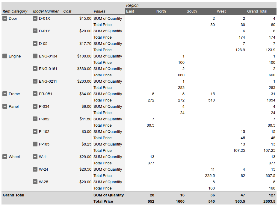
Add a pivot table with calculated values
The following
spreadsheets.batchUpdate
code sample shows how to use the
UpdateCellsRequest
to create a pivot table with a calculate values group from the source data,
anchoring it on cell A50 of the sheet specified by SHEET_ID.
The request configures the pivot table with the following properties:
- Two values groups (Quantity and Total Price). The first indicates the
number of sales. The second is a calculated value based on the product of a
part's cost and its total number of sales, using this formula:
=Cost*SUM(Quantity). - Three row groups (Item Category, Model Number, and Cost).
- One column group (Region).
- The row and column groups sort by name (rather than by Quantity) in each
group, alphabetizing the table. This is done by omitting the
valueBucketfield from thePivotGroup.- To simplify the table appearance, the request hides subtotals for all but the main row and column groups.
- The request sets
valueLayouttoVERTICALfor an improved table appearance.valueLayoutis only important if there's 2 or more value groups.
The request protocol is shown below.
POST https://sheets.googleapis.com/v4/spreadsheets/SPREADSHEET_ID:batchUpdate{
"requests": [
{
"updateCells": {
"rows": [
{
"values": [
{
"pivotTable": {
"source": {
"sheetId": SOURCE_SHEET_ID,
"startRowIndex": 0,
"startColumnIndex": 0,
"endRowIndex": 20,
"endColumnIndex": 7
},
"rows": [
{
"sourceColumnOffset": 0,
"showTotals": true,
"sortOrder": "ASCENDING"
},
{
"sourceColumnOffset": 1,
"showTotals": false,
"sortOrder": "ASCENDING",
},
{
"sourceColumnOffset": 2,
"showTotals": false,
"sortOrder": "ASCENDING",
}
],
"columns": [
{
"sourceColumnOffset": 4,
"sortOrder": "ASCENDING",
"showTotals": true
}
],
"values": [
{
"summarizeFunction": "SUM",
"sourceColumnOffset": 3
},
{
"summarizeFunction": "CUSTOM",
"name": "Total Price",
"formula": "=Cost*SUM(Quantity)"
}
],
"valueLayout": "VERTICAL"
}
}
]
}
],
"start": {
"sheetId": SHEET_ID,
"rowIndex": 49,
"columnIndex": 0
},
"fields": "pivotTable"
}
}
]
}The request creates a pivot table like this:
Delete a pivot table
The following
spreadsheets.batchUpdate
code sample shows how to use the
UpdateCellsRequest
to delete a pivot table (if present) that's anchored on cell A50 of the sheet
specified by SHEET_ID.
An UpdateCellsRequest can remove a pivot table by including "pivotTable" in
the fields parameter, while also omitting the pivotTable field on the anchor
cell.
The request protocol is shown below.
POST https://sheets.googleapis.com/v4/spreadsheets/SPREADSHEET_ID:batchUpdate{
"requests": [
{
"updateCells": {
"rows": [
{
"values": [
{}
]
}
],
"start": {
"sheetId": SHEET_ID,
"rowIndex": 49,
"columnIndex": 0
},
"fields": "pivotTable"
}
}
]
}Edit pivot table columns and rows
The following
spreadsheets.batchUpdate
code sample shows how to use the
UpdateCellsRequest
to edit the pivot table created in Add a pivot table.
Subsets of the
pivotTable
field in the
CellData resource
cannot be changed individually with the fields parameter. To make edits, the
entire pivotTable field must be supplied. Essentially, editing a pivot table
requires replacing it with a new one.
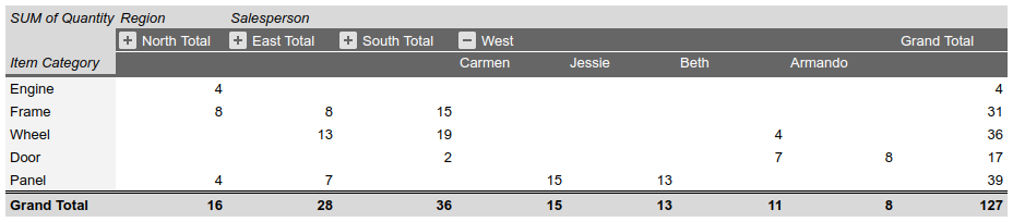
The request makes the following changes to the original pivot table:
- Removes the second row group from the original pivot table (Model Number).
- Adds a column group (Salesperson). The columns sort in descending order by the total number of Panel sales. "Carmen" (15 Panel sales) appears to the left of "Jessie" (13 Panel sales).
- Collapses the column for each Region, except for "West", hiding the
Salesperson group for that region. This is done by setting
collapsedtotruein thevalueMetadatafor that column in the Region column group.
The request protocol is shown below.
POST https://sheets.googleapis.com/v4/spreadsheets/SPREADSHEET_ID:batchUpdate{ "requests": [ { "updateCells": { "rows": [ { "values": [ { "pivotTable": { "source": { "sheetId":SOURCE_SHEET_ID, "startRowIndex": 0, "startColumnIndex": 0, "endRowIndex": 20, "endColumnIndex": 7 }, "rows": [ { "sourceColumnOffset": 0, "showTotals": true, "sortOrder": "ASCENDING", "valueBucket": { "buckets": [ { "stringValue": "West" } ] } } ], "columns": [ { "sourceColumnOffset": 4, "sortOrder": "ASCENDING", "showTotals": true, "valueBucket": {}, "valueMetadata": [ { "value": { "stringValue": "North" }, "collapsed": true }, { "value": { "stringValue": "South" }, "collapsed": true }, { "value": { "stringValue": "East" }, "collapsed": true } ] }, { "sourceColumnOffset": 5, "sortOrder": "DESCENDING", "showTotals": false, "valueBucket": { "buckets": [ { "stringValue": "Panel" } ] }, } ], "values": [ { "summarizeFunction": "SUM", "sourceColumnOffset": 3 } ], "valueLayout": "HORIZONTAL" } } ] } ], "start": { "sheetId":SHEET_ID, "rowIndex": 49, "columnIndex": 0 }, "fields": "pivotTable" } } ] }
The request creates a pivot table like this:
Read pivot table data
The following
spreadsheets.get code sample
shows how to get pivot table data from a spreadsheet. The fields query
parameter specifies that only the pivot table data should be returned (as
opposed to cell value data).
The request protocol is shown below.
GET https://sheets.googleapis.com/v4/spreadsheets/SPREADSHEET_ID?fields=sheets(properties.sheetId,data.rowData.values.pivotTable)The response consists of a
Spreadsheet
resource, which contains a
Sheet object with
SheetProperties
elements. There's also an array of
GridData
elements containing information about the
PivotTable.
Pivot table information is contained within the sheet's
CellData resource
for the cell that the table is anchored on (that is, the table's upper-left
corner). If a response field is set to the default value, it's omitted from the
response.
In this example, the first sheet (SOURCE_SHEET_ID) has the raw table
source data, while the second sheet (SHEET_ID) has the pivot table,
anchored on B3. The empty curly braces indicate sheets or cells that don't
contain pivot table data. For reference, this request also returns the sheet
IDs.
{ "sheets": [ { "data": [{}], "properties": { "sheetId":SOURCE_SHEET_ID} }, { "data": [ { "rowData": [ {}, {}, { "values": [ {}, { "pivotTable": { "columns": [ { "showTotals": true, "sortOrder": "ASCENDING", "sourceColumnOffset": 4, "valueBucket": {} } ], "rows": [ { "showTotals": true, "sortOrder": "ASCENDING", "valueBucket": { "buckets": [ { "stringValue": "West" } ] } }, { "showTotals": true, "sortOrder": "DESCENDING", "valueBucket": {}, "sourceColumnOffset": 1 } ], "source": { "sheetId":SOURCE_SHEET_ID, "startColumnIndex": 0, "endColumnIndex": 7, "startRowIndex": 0, "endRowIndex": 20 }, "values": [ { "sourceColumnOffset": 3, "summarizeFunction": "SUM" } ] } } ] } ] } ], "properties": { "sheetId":SHEET_ID} } ], }