
The Google Sheets API lets you create and update the conditional formatting rules in spreadsheets. Only certain formatting types (bold, italic, strikethrough, foreground color, and background color) can be controlled through conditional formatting. The examples on this page illustrate how to achieve common conditional formatting operations with the Sheets API.
These examples are presented as HTTP requests to be language neutral. To learn how to implement a batch update in different languages using the Google API client libraries, see Update spreadsheets.
In these examples, the placeholders SPREADSHEET_ID and
SHEET_ID indicates where you would provide those IDs. You can find
the spreadsheet ID in the
spreadsheet URL. You can get the sheet
ID by using the
spreadsheets.get
method. The ranges are specified using A1
notation. An example range is
Sheet1!A1:D5.
Add a conditional color gradient across a row
The following
spreadsheets.batchUpdate
method code sample shows how to use the
AddConditionalFormatRuleRequest
to establish new gradient conditional formatting rules for rows 10 and 11 of a
sheet. The first rule states that cells in that row have their background colors
set according to their value. The lowest value in the row is colored dark red,
while the highest value is colored bright green. The color of the other values
is interpolated. The second rule does the same, but with specific numeric values
determining the gradient endpoints (and different colors). The request uses the
sheets.InterpolationPointType
as the type.
The request protocol is shown below.
POST https://sheets.googleapis.com/v4/spreadsheets/SPREADSHEET_ID:batchUpdate
{
  "requests": [
    {
      "addConditionalFormatRule": {
        "rule": {
          "ranges": [
            {
              "sheetId": SHEET_ID,
              "startRowIndex": 9,
              "endRowIndex": 10,
            }
          ],
          "gradientRule": {
            "minpoint": {
              "color": {
                "green": 0.2,
                "red": 0.8
              },
              "type": "MIN"
            },
            "maxpoint": {
              "color": {
                "green": 0.9
              },
              "type": "MAX"
            },
          }
        },
        "index": 0
      }
    },
    {
      "addConditionalFormatRule": {
        "rule": {
          "ranges": [
            {
              "sheetId": SHEET_ID,
              "startRowIndex": 10,
              "endRowIndex": 11,
            }
          ],
          "gradientRule": {
            "minpoint": {
              "color": {
                "green": 0.8,
                "red": 0.8
              },
              "type": "NUMBER",
              "value": "0"
            },
            "maxpoint": {
              "color": {
                "blue": 0.9,
                "green": 0.5,
                "red": 0.5
              },
              "type": "NUMBER",
              "value": "256"
            },
          }
        },
        "index": 1
      }
    },
  ]
}
After the request, the applied format rule updates the sheet. Since the gradient
in row 11 has its maxpoint set to 256, any values above it have the maxpoint
color:

Add a conditional formatting rule to a set of ranges
The following
spreadsheets.batchUpdate
method code sample shows how to use the
AddConditionalFormatRuleRequest
to establish a new conditional formatting rule for columns A and C of a sheet.
The rule states that cells with values of 10 or less have their background
colors changed to a dark red. The rule is inserted at index 0, so it takes
priority over other formatting rules. The request uses the
ConditionType
as the type for the
BooleanRule.
The request protocol is shown below.
POST https://sheets.googleapis.com/v4/spreadsheets/SPREADSHEET_ID:batchUpdate
{
  "requests": [
    {
      "addConditionalFormatRule": {
        "rule": {
          "ranges": [
            {
              "sheetId": SHEET_ID,
              "startColumnIndex": 0,
              "endColumnIndex": 1,
            },
            {
              "sheetId": SHEET_ID,
              "startColumnIndex": 2,
              "endColumnIndex": 3,
            },
          ],
          "booleanRule": {
            "condition": {
              "type": "NUMBER_LESS_THAN_EQ",
              "values": [
                {
                  "userEnteredValue": "10"
                }
              ]
            },
            "format": {
              "backgroundColor": {
                "green": 0.2,
                "red": 0.8,
              }
            }
          }
        },
        "index": 0
      }
    }
  ]
}
After the request, the applied format rule updates the sheet:

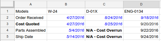
Add date and text conditional formatting rules to a range
The following
spreadsheets.batchUpdate
method code sample shows how to use the
AddConditionalFormatRuleRequest
to establish new conditional formatting rules for the range A1:D5 in a sheet,
based on date and text values in those cells. If the text contains the string
"Cost" (case-insensitive), the first rule sets the cell text as bold. If the
cell contains a date occurring before the past week, the second rule sets the
cell text as italics and colors it blue. The request uses the
ConditionType
as the type for the
BooleanRule.
The request protocol is shown below.
POST https://sheets.googleapis.com/v4/spreadsheets/SPREADSHEET_ID:batchUpdate
{
  "requests": [
    {
      "addConditionalFormatRule": {
        "rule": {
          "ranges": [
            {
              "sheetId": SHEET_ID,
              "startRowIndex": 0,
              "endRowIndex": 5,
              "startColumnIndex": 0,
              "endColumnIndex": 4,
            }
          ],
          "booleanRule": {
            "condition": {
              "type": "TEXT_CONTAINS",
              "values": [
                {
                  "userEnteredValue": "Cost"
                }
              ]
            },
            "format": {
              "textFormat": {
                "bold": true
              }
            }
          }
        },
        "index": 0
      }
    },
    {
      "addConditionalFormatRule": {
        "rule": {
          "ranges": [
            {
              "sheetId": SHEET_ID,
              "startRowIndex": 0,
              "endRowIndex": 5,
              "startColumnIndex": 0,
              "endColumnIndex": 4,
            }
          ],
          "booleanRule": {
            "condition": {
              "type": "DATE_BEFORE",
              "values": [
                {
                  "relativeDate": "PAST_WEEK"
                }
              ]
            },
            "format": {
              "textFormat": {
                "italic": true,
                "foregroundColor": {
                  "blue": 1
                }
              }
            }
          }
        },
        "index": 1
      }
    }
  ]
}
After the request, the applied format rule updates the sheet. In this example, the current date is 9/26/2016:
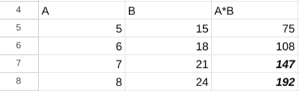
Add a custom formula rule to a range
The following
spreadsheets.batchUpdate
method code sample shows how to use the
AddConditionalFormatRuleRequest
to establish a new conditional formatting rule for the range B5:B8 in a sheet,
based on a custom formula. The rule calculates the product of the cell in
columns A and B. If the product is greater than 120, the cell text is set to
bold and italics. The request uses the
ConditionType
as the type for the
BooleanRule.
The request protocol is shown below.
POST https://sheets.googleapis.com/v4/spreadsheets/SPREADSHEET_ID:batchUpdate
{
  "requests": [
    {
      "addConditionalFormatRule": {
        "rule": {
          "ranges": [
            {
              "sheetId": SHEET_ID,
              "startColumnIndex": 2,
              "endColumnIndex": 3,
              "startRowIndex": 4,
              "endRowIndex": 8
            }
          ],
          "booleanRule": {
            "condition": {
              "type": "CUSTOM_FORMULA",
              "values": [
                {
                  "userEnteredValue": "=GT(A5*B5,120)"
                }
              ]
            },
            "format": {
              "textFormat": {
                "bold": true,
                "italic": true
              }
            }
          }
        },
        "index": 0
      }
    }
  ]
}
After the request, the applied format rule updates the sheet:
Delete a conditional formatting rule
The following
spreadsheets.batchUpdate
method code sample shows how to use the
DeleteConditionalFormatRuleRequest
to delete the conditional formatting rule with index 0 in the sheet specified
by SHEET_ID.
The request protocol is shown below.
POST https://sheets.googleapis.com/v4/spreadsheets/SPREADSHEET_ID:batchUpdate
{
  "requests": [
    {
      "deleteConditionalFormatRule": {
        "sheetId": SHEET_ID,
        "index": 0
      }
    }
  ]
}
Read the list of conditional formatting rules
The following
spreadsheets.get
method code sample shows how to get the title, SHEET_ID and list of
all conditional formatting rules for each sheet in a spreadsheet. The fields
query parameter determines what data to return.
The request protocol is shown below.
GET https://sheets.googleapis.com/v4/spreadsheets/SPREADSHEET_ID?fields=sheets(properties(title,sheetId),conditionalFormats)
The response consists of a
Spreadsheet resource,
which contains an array of
Sheet objects
each having a
SheetProperties
element and an array of
ConditionalFormatRule
elements. If a given response field is set to the default value, it's omitted
from the response. The request uses the
ConditionType
as the type for the
BooleanRule.
{
  "sheets": [
    {
      "properties": {
        "sheetId": 0,
        "title": "Sheet1"
      },
      "conditionalFormats": [
        {
          "ranges": [
            {
              "startRowIndex": 4,
              "endRowIndex": 8,
              "startColumnIndex": 2,
              "endColumnIndex": 3
            }
          ],
          "booleanRule": {
            "condition": {
              "type": "CUSTOM_FORMULA",
              "values": [
                {
                  "userEnteredValue": "=GT(A5*B5,120)"
                }
              ]
            },
            "format": {
              "textFormat": {
                "bold": true,
                "italic": true
              }
            }
          }
        },
        {
          "ranges": [
            {
              "startRowIndex": 0,
              "endRowIndex": 5,
              "startColumnIndex": 0,
              "endColumnIndex": 4
            }
          ],
          "booleanRule": {
            "condition": {
              "type": "DATE_BEFORE",
              "values": [
                {
                  "relativeDate": "PAST_WEEK"
                }
              ]
            },
            "format": {
              "textFormat": {
                "foregroundColor": {
                  "blue": 1
                },
                "italic": true
              }
            }
          }
        },
        ...
      ]
    }
  ]
}
Update a conditional formatting rule or its priority
The following
spreadsheets.batchUpdate
method code sample shows how to use the
UpdateConditionalFormatRuleRequest
with multiple requests. The first request moves an existing conditional format
rule to a higher index (from 0 to 2, decreasing its priority). The second
request replaces the conditional formatting rule at index 0 with a new rule
that formats cells containing the exact text specified ("Total Cost") in the
A1:D5 range. The first request's move is completed before the second begins, so
the second request is replacing the rule that was originally at index 1. The
request uses the
ConditionType
as the type for the
BooleanRule.
The request protocol is shown below.
POST https://sheets.googleapis.com/v4/spreadsheets/SPREADSHEET_ID:batchUpdate
{
  "requests": [
    {
      "updateConditionalFormatRule": {
        "sheetId": SHEET_ID,
        "index": 0,
        "newIndex": 2
      },
      "updateConditionalFormatRule": {
        "sheetId": SHEET_ID,
        "index": 0,
        "rule": {
          "ranges": [
            {
              "sheetId": SHEET_ID,
              "startRowIndex": 0,
              "endRowIndex": 5,
              "startColumnIndex": 0,
              "endColumnIndex": 4,
            }
          ],
          "booleanRule": {
            "condition": {
              "type": "TEXT_EQ",
              "values": [
                {
                  "userEnteredValue": "Total Cost"
                }
              ]
            },
            "format": {
              "textFormat": {
                "bold": true
              }
            }
          }
        }
      }
    }
  ]
}