
The Google Sheets API lets you create and update charts within spreadsheets as needed. The examples on this page illustrate how you can achieve some common chart operations with the Sheets API.
These examples are presented in the form of HTTP requests to be language neutral. To learn how to implement a batch update in different languages using the Google API client libraries, see Update spreadsheets.
In these examples, the placeholders SPREADSHEET_ID and SHEET_ID
indicates where you would provide those IDs. You can find the spreadsheet
ID in the spreadsheet URL.
You can get the sheet ID by using
the
spreadsheets.get
method. The ranges are specified using A1
notation. An example range is
Sheet1!A1:D5.
Additionally, the placeholder CHART_ID indicates the ID of a given
chart. You can set this ID when creating a chart with the Sheets API,
or allow Sheets API to generate one for you. You can get the IDs of
existing charts with the
spreadsheets.get
method.
Finally, the placeholder SOURCE_SHEET_ID indicates your sheet with the source data. In these examples, this is the table listed under Chart source data.
Chart source data
For these examples, assume the spreadsheet being used has the following source data in its first sheet ("Sheet1"). The strings in the first row are labels for the individual columns. To view examples of how to read from other sheets in your spreadsheet, see A1 notation.
| A | B | C | D | E | |
| 1 | Model Number | Sales - Jan | Sales - Feb | Sales - Mar | Total Sales |
| 2 | D-01X | 68 | 74 | 60 | 202 |
| 3 | FR-0B1 | 97 | 76 | 88 | 261 |
| 4 | P-034 | 27 | 49 | 32 | 108 |
| 5 | P-105 | 46 | 44 | 67 | 157 |
| 6 | W-11 | 75 | 68 | 87 | 230 |
| 7 | W-24 | 74 | 52 | 62 | 188 |
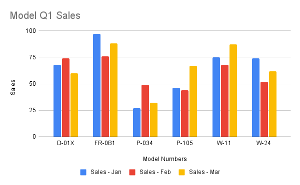
Add a column chart
The following
spreadsheets.batchUpdate
code sample shows how to use the
AddChartRequest
to create a column chart from the source data, placing it in a new sheet. The
request does the following to configure the chart:
- Sets the chart type as a column chart.
- Adds a legend to the bottom of the chart.
- Sets the chart and axis titles.
- Configures 3 data series, representing sales for 3 different months while using default formatting and colors.
The request protocol is shown below.
POST https://sheets.googleapis.com/v4/spreadsheets/SPREADSHEET_ID:batchUpdate
{
  "requests": [
    {
      "addChart": {
        "chart": {
          "spec": {
            "title": "Model Q1 Sales",
            "basicChart": {
              "chartType": "COLUMN",
              "legendPosition": "BOTTOM_LEGEND",
              "axis": [
                {
                  "position": "BOTTOM_AXIS",
                  "title": "Model Numbers"
                },
                {
                  "position": "LEFT_AXIS",
                  "title": "Sales"
                }
              ],
              "domains": [
                {
                  "domain": {
                    "sourceRange": {
                      "sources": [
                        {
                          "sheetId": SOURCE_SHEET_ID,
                          "startRowIndex": 0,
                          "endRowIndex": 7,
                          "startColumnIndex": 0,
                          "endColumnIndex": 1
                        }
                      ]
                    }
                  }
                }
              ],
              "series": [
                {
                  "series": {
                    "sourceRange": {
                      "sources": [
                        {
                          "sheetId": SOURCE_SHEET_ID,
                          "startRowIndex": 0,
                          "endRowIndex": 7,
                          "startColumnIndex": 1,
                          "endColumnIndex": 2
                        }
                      ]
                    }
                  },
                  "targetAxis": "LEFT_AXIS"
                },
                {
                  "series": {
                    "sourceRange": {
                      "sources": [
                        {
                          "sheetId": SOURCE_SHEET_ID,
                          "startRowIndex": 0,
                          "endRowIndex": 7,
                          "startColumnIndex": 2,
                          "endColumnIndex": 3
                        }
                      ]
                    }
                  },
                  "targetAxis": "LEFT_AXIS"
                },
                {
                  "series": {
                    "sourceRange": {
                      "sources": [
                        {
                          "sheetId": SOURCE_SHEET_ID,
                          "startRowIndex": 0,
                          "endRowIndex": 7,
                          "startColumnIndex": 3,
                          "endColumnIndex": 4
                        }
                      ]
                    }
                  },
                  "targetAxis": "LEFT_AXIS"
                }
              ],
              "headerCount": 1
            }
          },
          "position": {
            "newSheet": true
          }
        }
      }
    }
  ]
}
The request creates a chart in a new sheet like this:
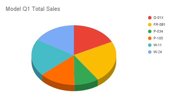
Add a pie chart
The following
spreadsheets.batchUpdate
code sample shows how to use the
AddChartRequest
to create a 3D pie chart from the source data. The request does the following to
configure the chart:
- Sets the chart title.
- Adds a legend to the right of the chart.
- Sets the chart as a 3D pie chart. Note that 3D pie charts cannot have a "donut hole" in the center the way flat pie charts can.
- Sets the chart data series as the total sales for each model number.
- Anchors the chart on cell C3 of the sheet specified by SHEET_ID, with a 50 pixel offset in both the X and Y directions.
The request protocol is shown below.
POST https://sheets.googleapis.com/v4/spreadsheets/SPREADSHEET_ID:batchUpdate
{
  "requests": [
    {
      "addChart": {
        "chart": {
          "spec": {
            "title": "Model Q1 Total Sales",
            "pieChart": {
              "legendPosition": "RIGHT_LEGEND",
              "threeDimensional": true,
              "domain": {
                "sourceRange": {
                  "sources": [
                    {
                      "sheetId": SOURCE_SHEET_ID,
                      "startRowIndex": 0,
                      "endRowIndex": 7,
                      "startColumnIndex": 0,
                      "endColumnIndex": 1
                    }
                  ]
                }
              },
              "series": {
                "sourceRange": {
                  "sources": [
                    {
                      "sheetId": SOURCE_SHEET_ID,
                      "startRowIndex": 0,
                      "endRowIndex": 7,
                      "startColumnIndex": 4,
                      "endColumnIndex": 5
                    }
                  ]
                }
              },
            }
          },
          "position": {
            "overlayPosition": {
              "anchorCell": {
                "sheetId": SHEET_ID,
                "rowIndex": 2,
                "columnIndex": 2
              },
              "offsetXPixels": 50,
              "offsetYPixels": 50
            }
          }
        }
      }
    }
  ]
}
The request creates a chart like this:
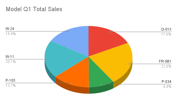
Alternatively, you can also update the legendPosition value from RIGHT_LEGEND to LABELED_LEGEND within the request so the legend values are connected to the pie chart slices.
'legendPosition': 'LABELED_LEGEND',
The updated request creates a chart like this:
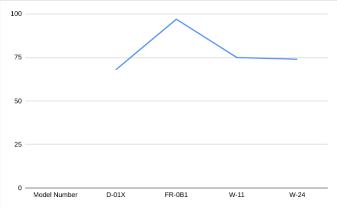
Add a line chart using multiple non-adjacent ranges
The following
spreadsheets.batchUpdate
code sample shows how to use the
AddChartRequest
to create a line chart from the source data, placing it in the source sheet.
Selecting non-adjacent ranges can be used to exclude rows from the
ChartSourceRange.
The request does the following to configure the chart:
- Sets the chart type as a line chart.
- Sets the horizontal x-axis title.
- Configures a data series representing sales. It sets A1:A3 and A6:A7 as a
domain, and B1:B3 and B6:B7 as aseries, while using default formatting and colors. Ranges are specified using A1 notation in the request URL. - Anchors the chart on cell H8 of the sheet specified by SHEET_ID.
The request protocol is shown below.
POST https://sheets.googleapis.com/v4/spreadsheets/SPREADSHEET_ID:batchUpdate
{
  "requests": [
    {
      "addChart": {
        "chart": {
          "spec": {
            "basicChart": {
              "chartType": "LINE",
              "domains": [
                {
                  "domain": {
                    "sourceRange": {
                      "sources": [
                        {
                          "startRowIndex": 0,
                          "endRowIndex": 3,
                          "startColumnIndex": 0,
                          "endColumnIndex": 1,
                          "sheetId": SOURCE_SHEET_ID
                        },
                        {
                          "startRowIndex": 5,
                          "endRowIndex": 7,
                          "startColumnIndex": 0,
                          "endColumnIndex": 1,
                          "sheetId": SOURCE_SHEET_ID
                        }
                      ]
                    }
                  }
                }
              ],
              "series": [
                {
                  "series": {
                    "sourceRange": {
                      "sources": [
                        {
                          "startRowIndex": 0,
                          "endRowIndex": 3,
                          "startColumnIndex": 1,
                          "endColumnIndex": 2,
                          "sheetId": SOURCE_SHEET_ID
                        },
                        {
                          "startRowIndex": 5,
                          "endRowIndex": 7,
                          "startColumnIndex": 1,
                          "endColumnIndex": 2,
                          "sheetId": SOURCE_SHEET_ID
                        }
                      ]
                    }
                  }
                }
              ]
            }
          },
          "position": {
            "overlayPosition": {
              "anchorCell": {
                "sheetId": SOURCE_SHEET_ID,
                "rowIndex": 8,
                "columnIndex": 8
              }
            }
          }
        }
      }
    }
  ]
}
The request creates a chart in a new sheet like this:
Delete a chart
The following
spreadsheets.batchUpdate
code sample shows how to use the
DeleteEmbeddedObjectRequest
to delete a chart specified by the CHART_ID.
The request protocol is shown below.
POST https://sheets.googleapis.com/v4/spreadsheets/SPREADSHEET_ID:batchUpdate
{
  "requests": [
    {
      "deleteEmbeddedObject": {
        "objectId": CHART_ID
      }
    }
  ]
}
Edit a chart's properties
The following
spreadsheets.batchUpdate
code sample shows how to use the
UpdateChartSpecRequest
to edit the chart created in the Add a column chart recipe,
modifying its data, type, and appearance. Subsets of chart properties cannot be
changed individually. To make edits, you must supply the entire spec field
with an UpdateChartSpecRequest. Essentially, editing a chart specification
requires replacing it with a new one.
The following request updates the original chart (specified by CHART_ID):
- Sets the chart type to
BAR. - Moves the legend to the right of the chart.
- Inverts the axes so that "Sales" is on the bottom axis and "Model Numbers" is on the left axis.
- Sets the axis title format to be 24-point font, bold, and italicized.
- Removes the "W-24" data from the chart (row 7 in chart source data).
The request protocol is shown below.
POST https://sheets.googleapis.com/v4/spreadsheets/SPREADSHEET_ID:batchUpdate
{
  "requests": [
    {
      "updateChartSpec": {
        "chartId": CHART_ID,
        "spec": {
          "title": "Model Q1 Sales",
          "basicChart": {
            "chartType": "BAR",
            "legendPosition": "RIGHT_LEGEND",
            "axis": [
              {
                "format": {
                  "bold": true,
                  "italic": true,
                  "fontSize": 24
                },
                "position": "BOTTOM_AXIS",
                "title": "Sales"
              },
              {
                "format": {
                  "bold": true,
                  "italic": true,
                  "fontSize": 24
                },
                "position": "LEFT_AXIS",
                "title": "Model Numbers"
              }
            ],
            "domains": [
              {
                "domain": {
                  "sourceRange": {
                    "sources": [
                      {
                        "sheetId": SOURCE_SHEET_ID,
                        "startRowIndex": 0,
                        "endRowIndex": 6,
                        "startColumnIndex": 0,
                        "endColumnIndex": 1
                      }
                    ]
                  }
                }
              }
            ],
            "series": [
              {
                "series": {
                  "sourceRange": {
                    "sources": [
                      {
                        "sheetId": SOURCE_SHEET_ID,
                        "startRowIndex": 0,
                        "endRowIndex": 6,
                        "startColumnIndex": 1,
                        "endColumnIndex": 2
                      }
                    ]
                  }
                },
                "targetAxis": "BOTTOM_AXIS"
              },
              {
                "series": {
                  "sourceRange": {
                    "sources": [
                      {
                        "sheetId": SOURCE_SHEET_ID,
                        "startRowIndex": 0,
                        "endRowIndex": 6,
                        "startColumnIndex": 2,
                        "endColumnIndex": 3
                      }
                    ]
                  }
                },
                "targetAxis": "BOTTOM_AXIS"
              },
              {
                "series": {
                  "sourceRange": {
                    "sources": [
                      {
                        "sheetId": SOURCE_SHEET_ID,
                        "startRowIndex": 0,
                        "endRowIndex": 6,
                        "startColumnIndex": 3,
                        "endColumnIndex": 4
                      }
                    ]
                  }
                },
                "targetAxis": "BOTTOM_AXIS"
              }
            ],
            "headerCount": 1
          }
        }
      }
    }
  ]
}
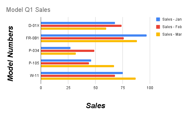
After the request the chart appears like this:
Move or resize a chart
The following
spreadsheets.batchUpdate
code sample shows how to use the
UpdateEmbeddedObjectPositionRequest
to move and resize a chart. After the request, the chart specified by CHART_ID
is:
- Anchored to cell A5 of its original sheet.
- Offset in the X direction by 100 pixels.
- Resized to 1200 by 742 pixels (the default size for a chart is 600 by 371 pixels).
The request only changes those properties specified with the fields parameter.
Other properties (such as offsetYPixels) retain their original values.
The request protocol is shown below.
POST https://sheets.googleapis.com/v4/spreadsheets/SPREADSHEET_ID:batchUpdate
{
  "requests": [
    {
      "updateEmbeddedObjectPosition": {
        "objectId": CHART_ID,
        "newPosition": {
          "overlayPosition": {
            "anchorCell": {
              "rowIndex": 4,
              "columnIndex": 0
            },
            "offsetXPixels": 100,
            "widthPixels": 1200,
            "heightPixels": 742
          }
        },
        "fields": "anchorCell(rowIndex,columnIndex),offsetXPixels,widthPixels,heightPixels"
      }
    }
  ]
}
Read chart data
The following
spreadsheets.get
code sample shows how to get chart data from a spreadsheet. The fields query
parameter specifies that only the chart data should be returned.
The response to this method call is a
spreadsheet
object, which contains an array of
sheet objects.
Any charts present on a sheet are represented in the
sheet object.
If a response field is set to the default value, it's omitted from the response.
In this example, the first sheet (SOURCE_SHEET_ID) doesn't have any charts, so an empty pair of curly braces is returned. The second sheet has the chart created by Add a column chart, and nothing else.
The request protocol is shown below.
GET https://sheets.googleapis.com/v4/spreadsheets/SPREADSHEET_ID?fields=sheets(charts)
{
  "sheets": [
    {},
    {
      "charts": [
        {
          "chartId": CHART_ID,
          "position": {
            "sheetId": SHEET_ID
          },
          "spec": {
            "basicChart": {
              "axis": [
                {
                  "format": {
                    "bold": false,
                    "italic": false
                  },
                  "position": "BOTTOM_AXIS",
                  "title": "Model Numbers"
                },
                {
                  "format": {
                    "bold": false,
                    "italic": false
                  },
                  "position": "LEFT_AXIS",
                  "title": "Sales"
                }
              ],
              "chartType": "COLUMN",
              "domains": [
                {
                  "domain": {
                    "sourceRange": {
                      "sources": [
                        {
                          "endColumnIndex": 1
                          "endRowIndex": 7,
                          "sheetId": SOURCE_SHEET_ID,
                          "startColumnIndex": 0,
                          "startRowIndex": 0,
                        }
                      ]
                    }
                  }
                }
              ],
              "legendPosition": "BOTTOM_LEGEND",
              "series": [
                {
                  "series": {
                    "sourceRange": {
                      "sources": [
                        {
                          "endColumnIndex": 2,
                          "endRowIndex": 7,
                          "sheetId": SOURCE_SHEET_ID,
                          "startColumnIndex": 1,
                          "startRowIndex": 0,
                        }
                      ]
                    }
                  },
                  "targetAxis": "LEFT_AXIS"
                },
                {
                  "series": {
                    "sourceRange": {
                      "sources": [
                        {
                          "endColumnIndex": 3,
                          "endRowIndex": 7,
                          "sheetId": SOURCE_SHEET_ID,
                          "startColumnIndex": 2,
                          "startRowIndex": 0,
                        }
                      ]
                    }
                  },
                  "targetAxis": "LEFT_AXIS"
                },
                {
                  "series": {
                    "sourceRange": {
                      "sources": [
                        {
                          "endColumnIndex": 4,
                          "endRowIndex": 7,
                          "sheetId": SOURCE_SHEET_ID,
                          "startColumnIndex": 3,
                          "startRowIndex": 0,
                        }
                      ]
                    }
                  },
                  "targetAxis": "LEFT_AXIS"
                }
              ]
            },
            "hiddenDimensionStrategy": "SKIP_HIDDEN_ROWS_AND_COLUMNS",
            "title": "Model Q1 Sales",
          },
        }
      ]
    }
  ]
}