Questa pagina è stata tradotta dall'API Cloud Translation.

Formattazione condizionale

La formattazione condizionale ti permette di formattare le celle in modo che il loro aspetto cambi dinamicamente in base al valore che contengono o ai valori di altre celle. Esistono molte possibili applicazioni della formattazione condizionale, tra cui i seguenti utilizzi:

Evidenzia le celle al di sopra di una determinata soglia (ad esempio, utilizzando il testo in grassetto per tutte le transazioni superiori a $2000).
Formatta le celle in modo che il colore vari con il loro valore (ad esempio, applicando uno sfondo rosso più intenso quando aumenta l'importo di oltre 2000 $).
Formatta dinamicamente le celle in base al contenuto di altre celle (ad esempio, evidenziando l'indirizzo delle proprietà il cui campo "time on market" è > 90 giorni).

Puoi anche formattare le celle in base al loro valore e a quelli di altre celle. Ad esempio, puoi formattare un intervallo di celle in base al loro valore rispetto al valore mediano dell'intervallo:

Formattazione per evidenziare i valori sopra o sotto l'età mediana.

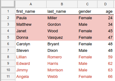
Figura 1. Formattazione per evidenziare i valori superiori o inferiori all'età mediana.

In questo esempio, le celle in ogni riga sono formattate in base al confronto tra il valore nella colonna age e il valore mediano di tutte le età. Le righe con età superiore alla mediana contengono testo rosso, mentre quelle al di sotto della media hanno uno sfondo rosso. Due delle righe hanno un valore per age che corrisponde all'età mediana (48) e queste celle non ricevono una formattazione speciale. Per il codice sorgente che crea questa formattazione condizionale, consulta l'esempio riportato di seguito.

Regole di formattazione condizionale

La formattazione condizionale viene espressa utilizzando le regole di formattazione. Ogni foglio di lavoro memorizza un elenco di queste regole e le applica nello stesso ordine in cui sono visualizzate nell'elenco. L'API Fogli Google consente di aggiungere, aggiornare ed eliminare queste regole di formattazione.

Ogni regola specifica un intervallo target, un tipo di regola, le condizioni per l'attivazione della regola e l'eventuale formattazione da applicare.

Intervallo di destinazione: può essere una singola cella, un intervallo di celle o più intervalli.

Tipo di regola: esistono due categorie di regole:

Le regole booleane applicano un formato solo se vengono soddisfatti criteri specifici.
Le regole della sfumatura calcolano il colore di sfondo di una cella, in base al valore della cella.

Le condizioni valutate e i formati che puoi applicare sono diversi per ciascuno di questi tipi di regole, come descritto nelle sezioni seguenti.

Regole booleane

Un BooleanRule definisce se applicare un formato specifico, in base a un BooleanCondition che restituisce true o false. Una regola booleana assume la forma:

{
  "condition": {
    object(BooleanCondition)
  },
  "format": {
    object(CellFormat)
  },
}

La condizione può utilizzare l'elemento ConditionType integrato oppure una formula personalizzata per valutazioni più complesse.

I tipi integrati ti consentono di applicare la formattazione in base a soglie numeriche, confronto del testo o al fatto che una cella sia compilata. Ad esempio, NUMBER_GREATER significa che il valore della cella deve essere maggiore del valore della condizione. Le regole vengono sempre valutate in base alla cella di destinazione.

La formula personalizzata è un tipo di condizione speciale che consente di applicare la formattazione in base a un'espressione arbitraria, il che consente anche la valutazione di qualsiasi cella, non solo della cella di destinazione. La formula della condizione deve restituire true.

Per definire la formattazione applicata da una regola booleana, utilizza un sottoinsieme del tipo CellFormat per definire:

Indica se il testo nella cella è in grassetto, corsivo o barrato.
Il colore del testo nella cella.
Il colore di sfondo della cella.

Utilizza solo le funzionalità di formattazione elencate sopra. Sebbene il tipo CellFormat possa esprimere altra formattazione, tra cui sottolineato, allineamento o bordi, un tentativo di utilizzo di questi elementi in una regola di formattazione condizionale genera un errore 400 invalid request.

Regole del gradiente

GradientRule definisce un intervallo di colori che corrisponde a un intervallo di valori. Una regola gradiente assume il seguente formato:

{
  "minpoint": {
    object(InterpolationPoint)
  },
  "midpoint": {
    object(InterpolationPoint)
  },
  "maxpoint": {
    object(InterpolationPoint)
  },
}

Ogni elemento InterpolationPoint definisce un colore e il valore corrispondente. Un insieme di tre punti definisce un gradiente di colore.

Gestire le regole di formattazione condizionale

Per creare, modificare o eliminare le regole di formattazione condizionale, utilizza il metodo spreadsheets.batchUpdate con il tipo di richiesta appropriato:

Aggiungi regole all'elenco nell'indice specificato utilizzando AddConditionalFormatRuleRequest.
Sostituisci o riordina le regole nell'elenco nell'indice specificato utilizzando UpdateConditionalFormatRuleRequest.
Rimuovi le regole dall'elenco nell'indice specificato utilizzando DeleteConditionalFormatRuleRequest.

Esempio

L'esempio seguente mostra come creare la formattazione condizionale mostrata nello screenshot nella parte superiore di questa pagina. Per ulteriori esempi, consulta la pagina di esempi della formattazione condizionale.

Apps Script

sheets/api/sheet_snippets.gs

Visualizza su GitHub

/**
 * conditional formatting
 * @param {string} spreadsheetId spreadsheet ID
 * @returns {*} spreadsheet
 */
Snippets.prototype.conditionalFormatting = (spreadsheetId) => {
  try {
    let myRange = Sheets.newGridRange();
    myRange.sheetId = 0;
    myRange.startRowIndex = 0;
    myRange.endRowIndex = 11;
    myRange.startColumnIndex = 0;
    myRange.endColumnIndex = 4;

    // Request 1
    let rule1ConditionalValue = Sheets.newConditionValue();
    rule1ConditionalValue.userEnteredValue = '=GT($D2,median($D$2:$D$11))';

    let rule1ConditionFormat = Sheets.newCellFormat();
    rule1ConditionFormat.textFormat = Sheets.newTextFormat();
    rule1ConditionFormat.textFormat.foregroundColor = Sheets.newColor();
    rule1ConditionFormat.textFormat.foregroundColor.red = 0.8;

    let rule1Condition = Sheets.newBooleanCondition();
    rule1Condition.type = 'CUSTOM_FORMULA';
    rule1Condition.values = [rule1ConditionalValue];

    let rule1BooleanRule = Sheets.newBooleanRule();
    rule1BooleanRule.condition = rule1Condition;
    rule1BooleanRule.format = rule1ConditionFormat;

    let rule1 = Sheets.newConditionalFormatRule();
    rule1.ranges = [myRange];
    rule1.booleanRule = rule1BooleanRule;

    let request1 = Sheets.newRequest();
    let addConditionalFormatRuleRequest1 =
      Sheets.newAddConditionalFormatRuleRequest();
    addConditionalFormatRuleRequest1.rule = rule1;
    addConditionalFormatRuleRequest1.index = 0;
    request1.addConditionalFormatRule = addConditionalFormatRuleRequest1;

    // Request 2
    let rule2ConditionalValue = Sheets.newConditionValue();
    rule2ConditionalValue.userEnteredValue = '=LT($D2,median($D$2:$D$11))';

    let rule2ConditionFormat = Sheets.newCellFormat();
    rule2ConditionFormat.textFormat = Sheets.newTextFormat();
    rule2ConditionFormat.textFormat.foregroundColor = Sheets.newColor();
    rule2ConditionFormat.textFormat.foregroundColor.red = 1;
    rule2ConditionFormat.textFormat.foregroundColor.green = 0.4;
    rule2ConditionFormat.textFormat.foregroundColor.blue = 0.4;

    let rule2Condition = Sheets.newBooleanCondition();
    rule2Condition.type = 'CUSTOM_FORMULA';
    rule2Condition.values = [rule2ConditionalValue];

    let rule2BooleanRule = Sheets.newBooleanRule();
    rule2BooleanRule.condition = rule2Condition;
    rule2BooleanRule.format = rule2ConditionFormat;

    let rule2 = Sheets.newConditionalFormatRule();
    rule2.ranges = [myRange];
    rule2.booleanRule = rule2BooleanRule;

    let request2 = Sheets.newRequest();
    let addConditionalFormatRuleRequest2 =
      Sheets.newAddConditionalFormatRuleRequest();
    addConditionalFormatRuleRequest2.rule = rule2;
    addConditionalFormatRuleRequest2.index = 0;
    request2.addConditionalFormatRule = addConditionalFormatRuleRequest2;

    // Batch send the requests
    const requests = [request1, request2];
    let batchUpdate = Sheets.newBatchUpdateSpreadsheetRequest();
    batchUpdate.requests = requests;
    const response =
      Sheets.Spreadsheets.batchUpdate(batchUpdate, spreadsheetId);
    return response;
  } catch (err) {
    // TODO (developer) - Handle exception
    console.log('Failed with error %s', err.message);
  }
};

Java

sheets/snippets/src/main/java/ConditionalFormatting.java

Visualizza su GitHub

import com.google.api.client.googleapis.json.GoogleJsonError;
import com.google.api.client.googleapis.json.GoogleJsonResponseException;
import com.google.api.client.http.HttpRequestInitializer;
import com.google.api.client.http.javanet.NetHttpTransport;
import com.google.api.client.json.gson.GsonFactory;
import com.google.api.services.sheets.v4.Sheets;
import com.google.api.services.sheets.v4.SheetsScopes;
import com.google.api.services.sheets.v4.model.AddConditionalFormatRuleRequest;
import com.google.api.services.sheets.v4.model.BatchUpdateSpreadsheetRequest;
import com.google.api.services.sheets.v4.model.BatchUpdateSpreadsheetResponse;
import com.google.api.services.sheets.v4.model.BooleanCondition;
import com.google.api.services.sheets.v4.model.BooleanRule;
import com.google.api.services.sheets.v4.model.CellFormat;
import com.google.api.services.sheets.v4.model.Color;
import com.google.api.services.sheets.v4.model.ConditionValue;
import com.google.api.services.sheets.v4.model.ConditionalFormatRule;
import com.google.api.services.sheets.v4.model.GridRange;
import com.google.api.services.sheets.v4.model.Request;
import com.google.api.services.sheets.v4.model.TextFormat;
import com.google.auth.http.HttpCredentialsAdapter;
import com.google.auth.oauth2.GoogleCredentials;
import java.io.IOException;
import java.util.Arrays;
import java.util.Collections;
import java.util.List;

/* Class to demonstrate the use of Spreadsheet Conditional Formatting API */
public class ConditionalFormatting {
  /**
   * Create conditional formatting.
   *
   * @param spreadsheetId - Id of the spreadsheet.
   * @return updated changes count.
   * @throws IOException - if credentials file not found.
   */
  public static BatchUpdateSpreadsheetResponse conditionalFormat(String spreadsheetId)
      throws IOException {
        /* Load pre-authorized user credentials from the environment.
           TODO(developer) - See https://developers.google.com/identity for
            guides on implementing OAuth2 for your application. */
    GoogleCredentials credentials = GoogleCredentials.getApplicationDefault()
        .createScoped(Collections.singleton(SheetsScopes.SPREADSHEETS));
    HttpRequestInitializer requestInitializer = new HttpCredentialsAdapter(
        credentials);

    // Create the sheets API client
    Sheets service = new Sheets.Builder(new NetHttpTransport(),
        GsonFactory.getDefaultInstance(),
        requestInitializer)
        .setApplicationName("Sheets samples")
        .build();

    List<GridRange> ranges = Collections.singletonList(new GridRange()
        .setSheetId(0)
        .setStartRowIndex(1)
        .setEndRowIndex(11)
        .setStartColumnIndex(0)
        .setEndColumnIndex(4)
    );
    List<Request> requests = Arrays.asList(
        new Request().setAddConditionalFormatRule(new AddConditionalFormatRuleRequest()
            .setRule(new ConditionalFormatRule()
                .setRanges(ranges)
                .setBooleanRule(new BooleanRule()
                    .setCondition(new BooleanCondition()
                        .setType("CUSTOM_FORMULA")
                        .setValues(Collections.singletonList(
                            new ConditionValue().setUserEnteredValue(
                                "=GT($D2,median($D$2:$D$11))")
                        ))
                    )
                    .setFormat(new CellFormat().setTextFormat(
                        new TextFormat().setForegroundColor(
                            new Color().setRed(0.8f))
                    ))
                )
            )
            .setIndex(0)
        ),
        new Request().setAddConditionalFormatRule(new AddConditionalFormatRuleRequest()
            .setRule(new ConditionalFormatRule()
                .setRanges(ranges)
                .setBooleanRule(new BooleanRule()
                    .setCondition(new BooleanCondition()
                        .setType("CUSTOM_FORMULA")
                        .setValues(Collections.singletonList(
                            new ConditionValue().setUserEnteredValue(
                                "=LT($D2,median($D$2:$D$11))")
                        ))
                    )
                    .setFormat(new CellFormat().setBackgroundColor(
                        new Color().setRed(1f).setGreen(0.4f).setBlue(0.4f)
                    ))
                )
            )
            .setIndex(0)
        )
    );

    BatchUpdateSpreadsheetResponse result = null;
    try {
      // Execute the requests.
      BatchUpdateSpreadsheetRequest body =
          new BatchUpdateSpreadsheetRequest()
              .setRequests(requests);
      result = service.spreadsheets()
          .batchUpdate(spreadsheetId, body)
          .execute();
      System.out.printf("%d cells updated.", result.getReplies().size());
    } catch (GoogleJsonResponseException e) {
      // TODO(developer) - handle error appropriately
      GoogleJsonError error = e.getDetails();
      if (error.getCode() == 404) {
        System.out.printf("Spreadsheet not found with id '%s'.\n", spreadsheetId);
      } else {
        throw e;
      }
    }
    return result;
  }
}

JavaScript

sheets/snippets/sheets_conditional_formatting.js

Visualizza su GitHub

function conditionalFormatting(spreadsheetId, callback) {
  const myRange = {
    sheetId: 0,
    startRowIndex: 1,
    endRowIndex: 11,
    startColumnIndex: 0,
    endColumnIndex: 4,
  };
  const requests = [{
    addConditionalFormatRule: {
      rule: {
        ranges: [myRange],
        booleanRule: {
          condition: {
            type: 'CUSTOM_FORMULA',
            values: [{userEnteredValue: '=GT($D2,median($D$2:$D$11))'}],
          },
          format: {
            textFormat: {foregroundColor: {red: 0.8}},
          },
        },
      },
      index: 0,
    },
  }, {
    addConditionalFormatRule: {
      rule: {
        ranges: [myRange],
        booleanRule: {
          condition: {
            type: 'CUSTOM_FORMULA',
            values: [{userEnteredValue: '=LT($D2,median($D$2:$D$11))'}],
          },
          format: {
            backgroundColor: {red: 1, green: 0.4, blue: 0.4},
          },
        },
      },
      index: 0,
    },
  }];

  const body = {
    requests,
  };
  try {
    gapi.client.sheets.spreadsheets.batchUpdate({
      spreadsheetId: spreadsheetId,
      resource: body,
    }).then((response) => {
      const result = response.result;
      console.log(`${result.replies.length} cells updated.`);
      if (callback) callback(response);
    });
  } catch (err) {
    document.getElementById('content').innerText = err.message;
    return;
  }
}

Node.js

sheets/snippets/sheets_conditional_formatting.js

Visualizza su GitHub

/**
 * Conditionally formats a Spreadsheet.
 * @param {string} spreadsheetId A Spreadsheet ID.
 * @return {obj} spreadsheet information
 */
async function conditionalFormatting(spreadsheetId) {
  const {GoogleAuth} = require('google-auth-library');
  const {google} = require('googleapis');

  const auth = new GoogleAuth({
    scopes: 'https://www.googleapis.com/auth/spreadsheets',
  });

  const service = google.sheets({version: 'v4', auth});
  const myRange = {
    sheetId: 0,
    startRowIndex: 1,
    endRowIndex: 11,
    startColumnIndex: 0,
    endColumnIndex: 4,
  };
  const requests = [
    {
      addConditionalFormatRule: {
        rule: {
          ranges: [myRange],
          booleanRule: {
            condition: {
              type: 'CUSTOM_FORMULA',
              values: [{userEnteredValue: '=GT($D2,median($D$2:$D$11))'}],
            },
            format: {
              textFormat: {foregroundColor: {red: 0.8}},
            },
          },
        },
        index: 0,
      },
    },
    {
      addConditionalFormatRule: {
        rule: {
          ranges: [myRange],
          booleanRule: {
            condition: {
              type: 'CUSTOM_FORMULA',
              values: [{userEnteredValue: '=LT($D2,median($D$2:$D$11))'}],
            },
            format: {
              backgroundColor: {red: 1, green: 0.4, blue: 0.4},
            },
          },
        },
        index: 0,
      },
    },
  ];
  const resource = {
    requests,
  };
  try {
    const response = await service.spreadsheets.batchUpdate({
      spreadsheetId,
      resource,
    });
    console.log(`${response.data.replies.length} cells updated.`);
    return response;
  } catch (err) {
    // TODO (developer) - Handle exception
    throw err;
  }
}

PHP

sheets/snippets/src/SpreadsheetConditionalFormatting.php

Visualizza su GitHub

use Google\Client;
use Google\Service\Drive;
use Google\Service\Sheets\BatchUpdateSpreadsheetRequest;
use Google\Service\Sheets\Request;

function conditionalFormatting($spreadsheetId)
    {
        /* Load pre-authorized user credentials from the environment.
           TODO(developer) - See https://developers.google.com/identity for
            guides on implementing OAuth2 for your application. */
        $client = new Google\Client();
        $client->useApplicationDefaultCredentials();
        $client->addScope(Google\Service\Drive::DRIVE);
        $service = new Google_Service_Sheets($client);

        try{
            $myRange = [
                'sheetId' => 0,
                'startRowIndex' => 1,
                'endRowIndex' => 11,
                'startColumnIndex' => 0,
                'endColumnIndex' => 4,
            ];
            //execute the request
            $requests = [
                new Google_Service_Sheets_Request([
                'addConditionalFormatRule' => [
                    'rule' => [
                        'ranges' => [ $myRange ],
                        'booleanRule' => [
                            'condition' => [
                                'type' => 'CUSTOM_FORMULA',
                                'values' => [ [ 'userEnteredValue' => '=GT($D2,median($D$2:$D$11))' ] ]
                            ],
                            'format' => [
                                'textFormat' => [ 'foregroundColor' => [ 'red' => 0.8 ] ]
                                ]
                                ]
                            ],
                            'index' => 0
                            ]
                        ]),
                        new Google_Service_Sheets_Request([
                'addConditionalFormatRule' => [
                    'rule' => [
                        'ranges' => [ $myRange ],
                        'booleanRule' => [
                            'condition' => [
                                'type' => 'CUSTOM_FORMULA',
                                'values' => [ [ 'userEnteredValue' => '=LT($D2,median($D$2:$D$11))' ] ]
                            ],
                            'format' => [
                                'backgroundColor' => [ 'red' => 1, 'green' => 0.4, 'blue' => 0.4 ]
                            ]
                            ]
                        ],
                    'index' => 0
                ]
                ])
        ];

        $batchUpdateRequest = new Google_Service_Sheets_BatchUpdateSpreadsheetRequest([
            'requests' => $requests
        ]);
        $response = $service->spreadsheets->batchUpdate($spreadsheetId, $batchUpdateRequest);
        printf("%d cells updated.", count($response->getReplies()));
        return $response;
    }
    catch(Exception $e) {
        // TODO(developer) - handle error appropriately
        echo 'Message: ' .$e->getMessage();
    }
}

Python

sheets/snippets/sheets_conditional_formatting.py

Visualizza su GitHub

import google.auth
from googleapiclient.discovery import build
from googleapiclient.errors import HttpError


def conditional_formatting(spreadsheet_id):
  """
  Creates the batch_update the user has access to.
  Load pre-authorized user credentials from the environment.
  TODO(developer) - See https://developers.google.com/identity
  for guides on implementing OAuth2 for the application.
  """
  creds, _ = google.auth.default()
  # pylint: disable=maybe-no-member
  try:
    service = build("sheets", "v4", credentials=creds)

    my_range = {
        "sheetId": 0,
        "startRowIndex": 1,
        "endRowIndex": 11,
        "startColumnIndex": 0,
        "endColumnIndex": 4,
    }
    requests = [
        {
            "addConditionalFormatRule": {
                "rule": {
                    "ranges": [my_range],
                    "booleanRule": {
                        "condition": {
                            "type": "CUSTOM_FORMULA",
                            "values": [
                                {
                                    "userEnteredValue": (
                                        "=GT($D2,median($D$2:$D$11))"
                                    )
                                }
                            ],
                        },
                        "format": {
                            "textFormat": {"foregroundColor": {"red": 0.8}}
                        },
                    },
                },
                "index": 0,
            }
        },
        {
            "addConditionalFormatRule": {
                "rule": {
                    "ranges": [my_range],
                    "booleanRule": {
                        "condition": {
                            "type": "CUSTOM_FORMULA",
                            "values": [
                                {
                                    "userEnteredValue": (
                                        "=LT($D2,median($D$2:$D$11))"
                                    )
                                }
                            ],
                        },
                        "format": {
                            "backgroundColor": {
                                "red": 1,
                                "green": 0.4,
                                "blue": 0.4,
                            }
                        },
                    },
                },
                "index": 0,
            }
        },
    ]
    body = {"requests": requests}
    response = (
        service.spreadsheets()
        .batchUpdate(spreadsheetId=spreadsheet_id, body=body)
        .execute()
    )
    print(f"{(len(response.get('replies')))} cells updated.")
    return response

  except HttpError as error:
    print(f"An error occurred: {error}")
    return error


if __name__ == "__main__":
  # Pass: spreadsheet_id
  conditional_formatting("1CM29gwKIzeXsAppeNwrc8lbYaVMmUclprLuLYuHog4k")

Ruby

sheets/snippets/lib/spreadsheet_snippets.rb

Visualizza su GitHub

my_range = {
  sheet_id:           0,
  start_row_index:    1,
  end_row_index:      11,
  start_column_index: 0,
  end_column_index:   4
}
requests = [{
  add_conditional_format_rule: {
    rule:  {
      ranges:       [my_range],
      boolean_rule: {
        condition: {
          type:   'CUSTOM_FORMULA',
          values: [{ user_entered_value: '=GT($D2,median($D$2:$D$11))' }]
        },
        format:    {
          text_format: { foreground_color: { red: 0.8 } }
        }
      }
    },
    index: 0
  }
}, {
  add_conditional_format_rule: {
    rule:  {
      ranges:       [my_range],
      boolean_rule: {
        condition: {
          type:   'CUSTOM_FORMULA',
          values: [{ user_entered_value: '=LT($D2,median($D$2:$D$11))' }]
        },
        format:    {
          background_color: { red: 1, green: 0.4, blue: 0.4 }
        }
      }
    },
    index: 0
  }
}]
body = {
  requests: requests
}
batch_update = Google::Apis::SheetsV4::BatchUpdateSpreadsheetRequest.new
batch_update.requests = requests
result = service.batch_update_spreadsheet(spreadsheet_id, batch_update)
puts "#{result.replies.length} cells updated."