सशर्त फ़ॉर्मेटिंग

कंडिशनल (शर्त के साथ) फ़ॉर्मैटिंग से सेल को फ़ॉर्मैट किया जा सकता है, ताकि वे उनमें मौजूद वैल्यू या दूसरी सेल की वैल्यू के हिसाब से डाइनैमिक तौर पर बदल सकें. कंडीशनल (शर्त के साथ) फ़ॉर्मैटिंग के कई इस्तेमाल हो सकते हैं. इनमें ये इस्तेमाल शामिल हैं:

  • किसी तय थ्रेशोल्ड से ज़्यादा की सेल को हाइलाइट करना. उदाहरण के लिए, 2,000 डॉलर से ज़्यादा के सभी लेन-देन के लिए बोल्ड टेक्स्ट का इस्तेमाल करना.
  • सेल को फ़ॉर्मैट करना, ताकि उनकी वैल्यू के मुताबिक उनका रंग अलग-अलग हो. उदाहरण के लिए, अगर 2,000 डॉलर से ज़्यादा की बढ़ोतरी होती है, तो ज़्यादा गहरे लाल रंग का बैकग्राउंड लागू किया जाता है.
  • दूसरे सेल के कॉन्टेंट के आधार पर सेल को डाइनैमिक तरीके से फ़ॉर्मैट करें. उदाहरण के लिए, उन प्रॉपर्टी के पते को हाइलाइट करना जिनका "मार्केट ऑन टाइम" फ़ील्ड > 90 दिन है.

सेल की वैल्यू और दूसरी सेल की वैल्यू के हिसाब से भी उन्हें फ़ॉर्मैट किया जा सकता है. उदाहरण के लिए, रेंज की मीडियन वैल्यू की तुलना में सेल की रेंज को उनकी वैल्यू के आधार पर फ़ॉर्मैट किया जा सकता है:

औसत उम्र से कम या ज़्यादा वाली वैल्यू को हाइलाइट करने के लिए फ़ॉर्मैट.

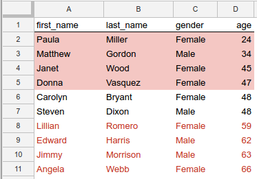
पहला डायग्राम. औसत उम्र से ज़्यादा या कम की वैल्यू को हाइलाइट करने के लिए फ़ॉर्मैट.

इस उदाहरण में, हर पंक्ति में मौजूद सेल को इस हिसाब से फ़ॉर्मैट किया जाता है कि उनके age कॉलम में मौजूद वैल्यू की तुलना सभी उम्र की मीडियन वैल्यू से कैसे की गई है. जिन पंक्तियों की उम्र मीडियन से ज़्यादा है, उनका टेक्स्ट लाल होता है. साथ ही, मीडियन के नीचे वाली लाइनों का बैकग्राउंड लाल होता है. दो पंक्तियों में से age के लिए ऐसी वैल्यू है जो मीडियन उम्र (48) से मेल खाती है. साथ ही, इन सेल को कोई खास फ़ॉर्मैट नहीं मिलता है. (इस कंडीशनल (शर्त के साथ) फ़ॉर्मैटिंग को बनाने वाले सोर्स कोड के लिए, नीचे दिया गया उदाहरण देखें.)

शर्त के साथ फ़ॉर्मैटिंग के नियम

कंडिशनल (शर्त के साथ) फ़ॉर्मैटिंग की सुविधा, फ़ॉर्मैट करने के नियमों का इस्तेमाल करके दिखाई जाती है. हर स्प्रेडशीट में इन नियमों की एक सूची सेव होती है और उन्हें उसी क्रम में लागू किया जाता है जिस क्रम में वे सूची में दिखते हैं. Google Sheets API से आप फ़ॉर्मैट करने के इन नियमों को जोड़ सकते हैं, अपडेट कर सकते हैं, और मिटा सकते हैं.

हर नियम में एक टारगेट रेंज, नियम का टाइप, नियम को ट्रिगर करने के लिए शर्तें, और लागू होने वाले फ़ॉर्मैट की जानकारी होती है.

टारगेट रेंज—यह कोई एक सेल, सेल की रेंज या कई रेंज हो सकती है.

नियम का टाइप—नियमों की दो कैटगरी होती हैं:

  • बूलियन नियम फ़ॉर्मैट सिर्फ़ तब लागू होते हैं, जब खास शर्तें पूरी होती हों.
  • ग्रेडिएंट के नियम, सेल की वैल्यू के आधार पर सेल के बैकग्राउंड के रंग का हिसाब लगाते हैं.

जिन शर्तों का आकलन किया जाता है और जो फ़ॉर्मैट लागू किए जा सकते हैं वे इनमें से हर नियम के टाइप के लिए अलग-अलग होती हैं, जैसा कि नीचे दिए गए सेक्शन में बताया गया है.

बूलियन नियम

BooleanRule से यह तय होता है कि किसी खास फ़ॉर्मैट को लागू करना है या नहीं. यह true या false के आकलन वाले BooleanCondition के आधार पर तय किया जाता है. बूलियन नियम इस रूप में होता है:

{
  "condition": {
    object(BooleanCondition)
  },
  "format": {
    object(CellFormat)
  },
}

शर्त, बिल्ट-इन ConditionType का इस्तेमाल कर सकती है या ज़्यादा मुश्किल आकलन करने के लिए, कस्टम फ़ॉर्मूला का इस्तेमाल कर सकती है.

पहले से मौजूद टाइप की मदद से, न्यूमेरिक थ्रेशोल्ड, टेक्स्ट की तुलना या सेल के हिसाब से फ़ॉर्मैटिंग लागू की जा सकती है. उदाहरण के लिए, NUMBER_GREATER का मतलब है कि सेल की वैल्यू, शर्त की वैल्यू से ज़्यादा होनी चाहिए. नियमों का हमेशा टारगेट सेल के आधार पर आकलन किया जाता है.

कस्टम फ़ॉर्मूला एक खास तरह की शर्त है. इसकी मदद से किसी आर्बिट्रेरी एक्सप्रेशन के मुताबिक फ़ॉर्मैटिंग लागू की जा सकती है. इससे सिर्फ़ टारगेट सेल के साथ-साथ किसी भी सेल का आकलन किया जा सकता है. शर्त के फ़ॉर्मूला की वैल्यू true पर सेट होनी चाहिए.

बूलियन नियम से लागू की गई फ़ॉर्मैटिंग को तय करने के लिए, आपको CellFormat टाइप के सबसेट का इस्तेमाल करना होगा:

  • सेल में मौजूद टेक्स्ट बोल्ड, इटैलिक या स्ट्राइकथ्रू है.
  • सेल में टेक्स्ट का रंग.
  • सेल का बैकग्राउंड रंग.

ग्रेडिएंट के नियम

A GradientRule वैल्यू की रेंज से जुड़े रंगों की रेंज के बारे में बताता है. ग्रेडिएंट नियम इस रूप में होता है:

{
  "minpoint": {
    object(InterpolationPoint)
  },
  "midpoint": {
    object(InterpolationPoint)
  },
  "maxpoint": {
    object(InterpolationPoint)
  },
}

हर InterpolationPoint, रंग और उससे जुड़ी वैल्यू के बारे में बताता है. तीन पॉइंट का सेट, कलर ग्रेडिएंट को तय करता है.

शर्त के साथ फ़ॉर्मैटिंग के नियमों को मैनेज करना

कंडीशनल (शर्त के साथ) फ़ॉर्मैटिंग के नियम बनाने, उनमें बदलाव करने या उन्हें मिटाने के लिए, सही अनुरोध टाइप के साथ spreadsheets.batchUpdate तरीके का इस्तेमाल करें:

  • AddConditionalFormatRuleRequest का इस्तेमाल करके, दिए गए इंडेक्स की सूची में नियम जोड़ें.

  • UpdateConditionalFormatRuleRequest का इस्तेमाल करके, दिए गए इंडेक्स की सूची में मौजूद नियमों को बदलें या उनका क्रम बदलें.

  • DeleteConditionalFormatRuleRequest का इस्तेमाल करके, दिए गए इंडेक्स की सूची से नियमों को हटाएं.

उदाहरण

नीचे दिए गए उदाहरण में, पेज पर सबसे ऊपर मौजूद स्क्रीनशॉट में दिखाए गए कंडिशनल (शर्त के साथ) फ़ॉर्मैटिंग को बनाने का तरीका बताया गया है. ज़्यादा उदाहरणों के लिए, शर्त वाली फ़ॉर्मैटिंग सैंपल वाला पेज देखें.

Apps Script

Sheets/api/स्प्रेडशीट_snippets.gs
/**
 * conditional formatting
 * @param {string} spreadsheetId spreadsheet ID
 * @returns {*} spreadsheet
 */
Snippets.prototype.conditionalFormatting = (spreadsheetId) => {
  try {
    let myRange = Sheets.newGridRange();
    myRange.sheetId = 0;
    myRange.startRowIndex = 0;
    myRange.endRowIndex = 11;
    myRange.startColumnIndex = 0;
    myRange.endColumnIndex = 4;

    // Request 1
    let rule1ConditionalValue = Sheets.newConditionValue();
    rule1ConditionalValue.userEnteredValue = '=GT($D2,median($D$2:$D$11))';

    let rule1ConditionFormat = Sheets.newCellFormat();
    rule1ConditionFormat.textFormat = Sheets.newTextFormat();
    rule1ConditionFormat.textFormat.foregroundColor = Sheets.newColor();
    rule1ConditionFormat.textFormat.foregroundColor.red = 0.8;

    let rule1Condition = Sheets.newBooleanCondition();
    rule1Condition.type = 'CUSTOM_FORMULA';
    rule1Condition.values = [rule1ConditionalValue];

    let rule1BooleanRule = Sheets.newBooleanRule();
    rule1BooleanRule.condition = rule1Condition;
    rule1BooleanRule.format = rule1ConditionFormat;

    let rule1 = Sheets.newConditionalFormatRule();
    rule1.ranges = [myRange];
    rule1.booleanRule = rule1BooleanRule;

    let request1 = Sheets.newRequest();
    let addConditionalFormatRuleRequest1 =
      Sheets.newAddConditionalFormatRuleRequest();
    addConditionalFormatRuleRequest1.rule = rule1;
    addConditionalFormatRuleRequest1.index = 0;
    request1.addConditionalFormatRule = addConditionalFormatRuleRequest1;

    // Request 2
    let rule2ConditionalValue = Sheets.newConditionValue();
    rule2ConditionalValue.userEnteredValue = '=LT($D2,median($D$2:$D$11))';

    let rule2ConditionFormat = Sheets.newCellFormat();
    rule2ConditionFormat.textFormat = Sheets.newTextFormat();
    rule2ConditionFormat.textFormat.foregroundColor = Sheets.newColor();
    rule2ConditionFormat.textFormat.foregroundColor.red = 1;
    rule2ConditionFormat.textFormat.foregroundColor.green = 0.4;
    rule2ConditionFormat.textFormat.foregroundColor.blue = 0.4;

    let rule2Condition = Sheets.newBooleanCondition();
    rule2Condition.type = 'CUSTOM_FORMULA';
    rule2Condition.values = [rule2ConditionalValue];

    let rule2BooleanRule = Sheets.newBooleanRule();
    rule2BooleanRule.condition = rule2Condition;
    rule2BooleanRule.format = rule2ConditionFormat;

    let rule2 = Sheets.newConditionalFormatRule();
    rule2.ranges = [myRange];
    rule2.booleanRule = rule2BooleanRule;

    let request2 = Sheets.newRequest();
    let addConditionalFormatRuleRequest2 =
      Sheets.newAddConditionalFormatRuleRequest();
    addConditionalFormatRuleRequest2.rule = rule2;
    addConditionalFormatRuleRequest2.index = 0;
    request2.addConditionalFormatRule = addConditionalFormatRuleRequest2;

    // Batch send the requests
    const requests = [request1, request2];
    let batchUpdate = Sheets.newBatchUpdateSpreadsheetRequest();
    batchUpdate.requests = requests;
    const response =
      Sheets.Spreadsheets.batchUpdate(batchUpdate, spreadsheetId);
    return response;
  } catch (err) {
    // TODO (developer) - Handle exception
    console.log('Failed with error %s', err.message);
  }
};

Java

sheets/snippets/src/main/java/ConditionalFormatting.java
import com.google.api.client.googleapis.json.GoogleJsonError;
import com.google.api.client.googleapis.json.GoogleJsonResponseException;
import com.google.api.client.http.HttpRequestInitializer;
import com.google.api.client.http.javanet.NetHttpTransport;
import com.google.api.client.json.gson.GsonFactory;
import com.google.api.services.sheets.v4.Sheets;
import com.google.api.services.sheets.v4.SheetsScopes;
import com.google.api.services.sheets.v4.model.AddConditionalFormatRuleRequest;
import com.google.api.services.sheets.v4.model.BatchUpdateSpreadsheetRequest;
import com.google.api.services.sheets.v4.model.BatchUpdateSpreadsheetResponse;
import com.google.api.services.sheets.v4.model.BooleanCondition;
import com.google.api.services.sheets.v4.model.BooleanRule;
import com.google.api.services.sheets.v4.model.CellFormat;
import com.google.api.services.sheets.v4.model.Color;
import com.google.api.services.sheets.v4.model.ConditionValue;
import com.google.api.services.sheets.v4.model.ConditionalFormatRule;
import com.google.api.services.sheets.v4.model.GridRange;
import com.google.api.services.sheets.v4.model.Request;
import com.google.api.services.sheets.v4.model.TextFormat;
import com.google.auth.http.HttpCredentialsAdapter;
import com.google.auth.oauth2.GoogleCredentials;
import java.io.IOException;
import java.util.Arrays;
import java.util.Collections;
import java.util.List;

/* Class to demonstrate the use of Spreadsheet Conditional Formatting API */
public class ConditionalFormatting {
  /**
   * Create conditional formatting.
   *
   * @param spreadsheetId - Id of the spreadsheet.
   * @return updated changes count.
   * @throws IOException - if credentials file not found.
   */
  public static BatchUpdateSpreadsheetResponse conditionalFormat(String spreadsheetId)
      throws IOException {
        /* Load pre-authorized user credentials from the environment.
           TODO(developer) - See https://developers.google.com/identity for
            guides on implementing OAuth2 for your application. */
    GoogleCredentials credentials = GoogleCredentials.getApplicationDefault()
        .createScoped(Collections.singleton(SheetsScopes.SPREADSHEETS));
    HttpRequestInitializer requestInitializer = new HttpCredentialsAdapter(
        credentials);

    // Create the sheets API client
    Sheets service = new Sheets.Builder(new NetHttpTransport(),
        GsonFactory.getDefaultInstance(),
        requestInitializer)
        .setApplicationName("Sheets samples")
        .build();

    List<GridRange> ranges = Collections.singletonList(new GridRange()
        .setSheetId(0)
        .setStartRowIndex(1)
        .setEndRowIndex(11)
        .setStartColumnIndex(0)
        .setEndColumnIndex(4)
    );
    List<Request> requests = Arrays.asList(
        new Request().setAddConditionalFormatRule(new AddConditionalFormatRuleRequest()
            .setRule(new ConditionalFormatRule()
                .setRanges(ranges)
                .setBooleanRule(new BooleanRule()
                    .setCondition(new BooleanCondition()
                        .setType("CUSTOM_FORMULA")
                        .setValues(Collections.singletonList(
                            new ConditionValue().setUserEnteredValue(
                                "=GT($D2,median($D$2:$D$11))")
                        ))
                    )
                    .setFormat(new CellFormat().setTextFormat(
                        new TextFormat().setForegroundColor(
                            new Color().setRed(0.8f))
                    ))
                )
            )
            .setIndex(0)
        ),
        new Request().setAddConditionalFormatRule(new AddConditionalFormatRuleRequest()
            .setRule(new ConditionalFormatRule()
                .setRanges(ranges)
                .setBooleanRule(new BooleanRule()
                    .setCondition(new BooleanCondition()
                        .setType("CUSTOM_FORMULA")
                        .setValues(Collections.singletonList(
                            new ConditionValue().setUserEnteredValue(
                                "=LT($D2,median($D$2:$D$11))")
                        ))
                    )
                    .setFormat(new CellFormat().setBackgroundColor(
                        new Color().setRed(1f).setGreen(0.4f).setBlue(0.4f)
                    ))
                )
            )
            .setIndex(0)
        )
    );

    BatchUpdateSpreadsheetResponse result = null;
    try {
      // Execute the requests.
      BatchUpdateSpreadsheetRequest body =
          new BatchUpdateSpreadsheetRequest()
              .setRequests(requests);
      result = service.spreadsheets()
          .batchUpdate(spreadsheetId, body)
          .execute();
      System.out.printf("%d cells updated.", result.getReplies().size());
    } catch (GoogleJsonResponseException e) {
      // TODO(developer) - handle error appropriately
      GoogleJsonError error = e.getDetails();
      if (error.getCode() == 404) {
        System.out.printf("Spreadsheet not found with id '%s'.\n", spreadsheetId);
      } else {
        throw e;
      }
    }
    return result;
  }
}

JavaScript

sheets/snippets/sheets_conditional_formatting.js
function conditionalFormatting(spreadsheetId, callback) {
  const myRange = {
    sheetId: 0,
    startRowIndex: 1,
    endRowIndex: 11,
    startColumnIndex: 0,
    endColumnIndex: 4,
  };
  const requests = [{
    addConditionalFormatRule: {
      rule: {
        ranges: [myRange],
        booleanRule: {
          condition: {
            type: 'CUSTOM_FORMULA',
            values: [{userEnteredValue: '=GT($D2,median($D$2:$D$11))'}],
          },
          format: {
            textFormat: {foregroundColor: {red: 0.8}},
          },
        },
      },
      index: 0,
    },
  }, {
    addConditionalFormatRule: {
      rule: {
        ranges: [myRange],
        booleanRule: {
          condition: {
            type: 'CUSTOM_FORMULA',
            values: [{userEnteredValue: '=LT($D2,median($D$2:$D$11))'}],
          },
          format: {
            backgroundColor: {red: 1, green: 0.4, blue: 0.4},
          },
        },
      },
      index: 0,
    },
  }];

  const body = {
    requests,
  };
  try {
    gapi.client.sheets.spreadsheets.batchUpdate({
      spreadsheetId: spreadsheetId,
      resource: body,
    }).then((response) => {
      const result = response.result;
      console.log(`${result.replies.length} cells updated.`);
      if (callback) callback(response);
    });
  } catch (err) {
    document.getElementById('content').innerText = err.message;
    return;
  }
}

Node.js

sheets/snippets/sheets_conditional_formatting.js
/**
 * Conditionally formats a Spreadsheet.
 * @param {string} spreadsheetId A Spreadsheet ID.
 * @return {obj} spreadsheet information
 */
async function conditionalFormatting(spreadsheetId) {
  const {GoogleAuth} = require('google-auth-library');
  const {google} = require('googleapis');

  const auth = new GoogleAuth({
    scopes: 'https://www.googleapis.com/auth/spreadsheets',
  });

  const service = google.sheets({version: 'v4', auth});
  const myRange = {
    sheetId: 0,
    startRowIndex: 1,
    endRowIndex: 11,
    startColumnIndex: 0,
    endColumnIndex: 4,
  };
  const requests = [
    {
      addConditionalFormatRule: {
        rule: {
          ranges: [myRange],
          booleanRule: {
            condition: {
              type: 'CUSTOM_FORMULA',
              values: [{userEnteredValue: '=GT($D2,median($D$2:$D$11))'}],
            },
            format: {
              textFormat: {foregroundColor: {red: 0.8}},
            },
          },
        },
        index: 0,
      },
    },
    {
      addConditionalFormatRule: {
        rule: {
          ranges: [myRange],
          booleanRule: {
            condition: {
              type: 'CUSTOM_FORMULA',
              values: [{userEnteredValue: '=LT($D2,median($D$2:$D$11))'}],
            },
            format: {
              backgroundColor: {red: 1, green: 0.4, blue: 0.4},
            },
          },
        },
        index: 0,
      },
    },
  ];
  const resource = {
    requests,
  };
  try {
    const response = await service.spreadsheets.batchUpdate({
      spreadsheetId,
      resource,
    });
    console.log(`${response.data.replies.length} cells updated.`);
    return response;
  } catch (err) {
    // TODO (developer) - Handle exception
    throw err;
  }
}

PHP

sheets/snippets/src/SpreadsheetConditionalFormatting.php
use Google\Client;
use Google\Service\Drive;
use Google\Service\Sheets\BatchUpdateSpreadsheetRequest;
use Google\Service\Sheets\Request;

function conditionalFormatting($spreadsheetId)
    {
        /* Load pre-authorized user credentials from the environment.
           TODO(developer) - See https://developers.google.com/identity for
            guides on implementing OAuth2 for your application. */
        $client = new Google\Client();
        $client->useApplicationDefaultCredentials();
        $client->addScope(Google\Service\Drive::DRIVE);
        $service = new Google_Service_Sheets($client);

        try{
            $myRange = [
                'sheetId' => 0,
                'startRowIndex' => 1,
                'endRowIndex' => 11,
                'startColumnIndex' => 0,
                'endColumnIndex' => 4,
            ];
            //execute the request
            $requests = [
                new Google_Service_Sheets_Request([
                'addConditionalFormatRule' => [
                    'rule' => [
                        'ranges' => [ $myRange ],
                        'booleanRule' => [
                            'condition' => [
                                'type' => 'CUSTOM_FORMULA',
                                'values' => [ [ 'userEnteredValue' => '=GT($D2,median($D$2:$D$11))' ] ]
                            ],
                            'format' => [
                                'textFormat' => [ 'foregroundColor' => [ 'red' => 0.8 ] ]
                                ]
                                ]
                            ],
                            'index' => 0
                            ]
                        ]),
                        new Google_Service_Sheets_Request([
                'addConditionalFormatRule' => [
                    'rule' => [
                        'ranges' => [ $myRange ],
                        'booleanRule' => [
                            'condition' => [
                                'type' => 'CUSTOM_FORMULA',
                                'values' => [ [ 'userEnteredValue' => '=LT($D2,median($D$2:$D$11))' ] ]
                            ],
                            'format' => [
                                'backgroundColor' => [ 'red' => 1, 'green' => 0.4, 'blue' => 0.4 ]
                            ]
                            ]
                        ],
                    'index' => 0
                ]
                ])
        ];

        $batchUpdateRequest = new Google_Service_Sheets_BatchUpdateSpreadsheetRequest([
            'requests' => $requests
        ]);
        $response = $service->spreadsheets->batchUpdate($spreadsheetId, $batchUpdateRequest);
        printf("%d cells updated.", count($response->getReplies()));
        return $response;
    }
    catch(Exception $e) {
        // TODO(developer) - handle error appropriately
        echo 'Message: ' .$e->getMessage();
    }
}

Python

sheets/snippets/sheets_conditional_formatting.py
import google.auth
from googleapiclient.discovery import build
from googleapiclient.errors import HttpError


def conditional_formatting(spreadsheet_id):
  """
  Creates the batch_update the user has access to.
  Load pre-authorized user credentials from the environment.
  TODO(developer) - See https://developers.google.com/identity
  for guides on implementing OAuth2 for the application.
  """
  creds, _ = google.auth.default()
  # pylint: disable=maybe-no-member
  try:
    service = build("sheets", "v4", credentials=creds)

    my_range = {
        "sheetId": 0,
        "startRowIndex": 1,
        "endRowIndex": 11,
        "startColumnIndex": 0,
        "endColumnIndex": 4,
    }
    requests = [
        {
            "addConditionalFormatRule": {
                "rule": {
                    "ranges": [my_range],
                    "booleanRule": {
                        "condition": {
                            "type": "CUSTOM_FORMULA",
                            "values": [
                                {
                                    "userEnteredValue": (
                                        "=GT($D2,median($D$2:$D$11))"
                                    )
                                }
                            ],
                        },
                        "format": {
                            "textFormat": {"foregroundColor": {"red": 0.8}}
                        },
                    },
                },
                "index": 0,
            }
        },
        {
            "addConditionalFormatRule": {
                "rule": {
                    "ranges": [my_range],
                    "booleanRule": {
                        "condition": {
                            "type": "CUSTOM_FORMULA",
                            "values": [
                                {
                                    "userEnteredValue": (
                                        "=LT($D2,median($D$2:$D$11))"
                                    )
                                }
                            ],
                        },
                        "format": {
                            "backgroundColor": {
                                "red": 1,
                                "green": 0.4,
                                "blue": 0.4,
                            }
                        },
                    },
                },
                "index": 0,
            }
        },
    ]
    body = {"requests": requests}
    response = (
        service.spreadsheets()
        .batchUpdate(spreadsheetId=spreadsheet_id, body=body)
        .execute()
    )
    print(f"{(len(response.get('replies')))} cells updated.")
    return response

  except HttpError as error:
    print(f"An error occurred: {error}")
    return error


if __name__ == "__main__":
  # Pass: spreadsheet_id
  conditional_formatting("1CM29gwKIzeXsAppeNwrc8lbYaVMmUclprLuLYuHog4k")

Ruby

sheets/snippets/lib/spreadsheet_snippets.rb
my_range = {
  sheet_id:           0,
  start_row_index:    1,
  end_row_index:      11,
  start_column_index: 0,
  end_column_index:   4
}
requests = [{
  add_conditional_format_rule: {
    rule:  {
      ranges:       [my_range],
      boolean_rule: {
        condition: {
          type:   'CUSTOM_FORMULA',
          values: [{ user_entered_value: '=GT($D2,median($D$2:$D$11))' }]
        },
        format:    {
          text_format: { foreground_color: { red: 0.8 } }
        }
      }
    },
    index: 0
  }
}, {
  add_conditional_format_rule: {
    rule:  {
      ranges:       [my_range],
      boolean_rule: {
        condition: {
          type:   'CUSTOM_FORMULA',
          values: [{ user_entered_value: '=LT($D2,median($D$2:$D$11))' }]
        },
        format:    {
          background_color: { red: 1, green: 0.4, blue: 0.4 }
        }
      }
    },
    index: 0
  }
}]
body = {
  requests: requests
}
batch_update = Google::Apis::SheetsV4::BatchUpdateSpreadsheetRequest.new
batch_update.requests = requests
result = service.batch_update_spreadsheet(spreadsheet_id, batch_update)
puts "#{result.replies.length} cells updated."