В этом глоссарии даны определения терминов, связанных с искусственным интеллектом.
А
абляция
Метод оценки важности признака или компонента путем его временного удаления из модели . Затем модель переобучается без этого признака или компонента, и если переобученная модель показывает значительно худшие результаты, то удаленный признак или компонент, вероятно, был важен.
Например, предположим, вы обучили модель классификации на 10 признаках и достигли точности 88% на тестовом наборе . Чтобы проверить важность первого признака, вы можете переобучить модель, используя только девять других признаков. Если переобученная модель показывает значительно худшие результаты (например, точность 55%), то, вероятно, удаленный признак был важен. И наоборот, если переобученная модель показывает такие же хорошие результаты, то, вероятно, этот признак был не так уж важен.
Абляция также может помочь определить значимость следующих факторов:
- Более крупные компоненты, такие как целая подсистема более крупной системы машинного обучения.
- Процессы или методы, например, этап предварительной обработки данных.
В обоих случаях вы сможете наблюдать, как изменяется (или не изменяется) производительность системы после удаления компонента.
A/B-тестирование
Статистический способ сравнения двух (или более) методов — A и B. Как правило, A — это уже существующий метод, а B — новый. A/B-тестирование позволяет не только определить, какой метод работает лучше, но и выяснить, является ли разница статистически значимой.
A/B-тестирование обычно сравнивает один показатель по двум методам; например, как точность модели соотносится с точностью двух методов? Однако A/B-тестирование может также сравнивать любое конечное число показателей.
чип-ускоритель
Категория специализированных аппаратных компонентов, предназначенных для выполнения ключевых вычислений, необходимых для алгоритмов глубокого обучения.
Ускорительные чипы (или просто ускорители ) могут значительно повысить скорость и эффективность задач обучения и вывода по сравнению с центральным процессором общего назначения. Они идеально подходят для обучения нейронных сетей и аналогичных ресурсоемких вычислительных задач.
Примерами микросхем-ускорителей являются:
- Тензорные процессоры Google ( TPU ) со специализированным оборудованием для глубокого обучения.
- Графические процессоры NVIDIA, хотя и были изначально разработаны для обработки графики, позволяют использовать параллельную обработку, что может значительно повысить скорость обработки.
точность
Количество правильных классификационных прогнозов, деленное на общее количество прогнозов. То есть:
Например, модель, сделавшая 40 правильных и 10 неправильных прогнозов, будет иметь точность:
Бинарная классификация предоставляет конкретные названия для различных категорий правильных и неправильных прогнозов . Таким образом, формула точности для бинарной классификации выглядит следующим образом:
где:
- TP — это количество истинно положительных результатов (правильных прогнозов).
- TN — это количество истинно отрицательных результатов (правильных предсказаний).
- FP — это количество ложноположительных результатов (неверных прогнозов).
- FN — это количество ложноотрицательных результатов (неверных прогнозов).
Сравните и сопоставьте точность с прецизией и полнотой .
Дополнительную информацию см. в разделе «Классификация: точность, полнота, прецизионность и связанные с ними показатели» в кратком курсе по машинному обучению.
действовать
Этап в цикле работы агента, на котором агент выполняет действие, выбранное на этапе обоснования . Например, на этапе выполнения действия может быть отправлен API-запрос.
действие
В обучении с подкреплением механизм, посредством которого агент переходит между состояниями окружающей среды , заключается в выборе действия с использованием стратегии .
пространство действий
Пространство действий — это набор ресурсов, которые агент может использовать для выполнения задачи. В него могут входить инструменты и API, которые агент может вызывать, а также его права доступа. В целом, пространство действий должно быть достаточно большим, чтобы агент мог выполнить задачу. Если пространство действий слишком мало, у агента может не хватать ресурсов для выполнения задачи. Если же пространство действий слишком велико, агент, как правило, становится более склонен к ошибкам.
функция активации
Функция, позволяющая нейронным сетям изучать нелинейные (сложные) взаимосвязи между признаками и меткой.
К популярным функциям активации относятся:
Графики функций активации никогда не представляют собой одну прямую линию. Например, график функции активации ReLU состоит из двух прямых линий:

График сигмоидной функции активации выглядит следующим образом:

Нажмите на значок, чтобы увидеть пример.
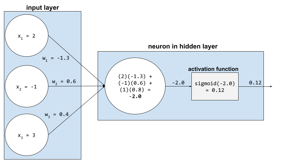
В нейронной сети функции активации обрабатывают взвешенную сумму всех входных сигналов нейрона . Для вычисления взвешенной суммы нейрон суммирует произведения соответствующих значений и весов. Например, предположим, что соответствующие входные сигналы для нейрона состоят из следующего:
| входное значение | входной вес |
| 2 | -1.3 |
| -1 | 0,6 |
| 3 | 0,4 |
weighted sum = (2)(-1.3) + (-1)(0.6) + (3)(0.4) = -2.0
Дополнительную информацию можно найти в разделе «Нейронные сети: функции активации» в кратком курсе по машинному обучению.
активное обучение
Активное обучение — это подход к обучению , при котором алгоритм выбирает часть данных, на которых он обучается. Оно особенно ценно, когда размеченные примеры редки или их получение обходится дорого. Вместо того чтобы слепо искать разнообразный набор размеченных примеров, алгоритм активного обучения избирательно ищет именно тот набор примеров, который ему необходим для обучения.
АдаГрад
Сложный алгоритм градиентного спуска, который масштабирует градиенты каждого параметра , фактически задавая каждому параметру независимую скорость обучения . Подробное объяснение см. в разделе «Адаптивные субградиентные методы для онлайн-обучения и стохастической оптимизации» .
приспособление
Синоним к слову «настройка» или «тонкая настройка» .
агент
Программное обеспечение, способное анализировать вводимые пользователем данные для планирования и выполнения действий от его имени.
В обучении с подкреплением агент — это сущность, которая использует стратегию для максимизации ожидаемой отдачи от перехода между состояниями окружающей среды .
агентный
Прилагательная форма слова «агент» . «Агентный» относится к качествам, которыми обладают агенты (например, автономия).
агентный цикл
Цикл, который агент проходит до тех пор, пока не будет выполнено условие завершения . Цикл обычно состоит из следующих четырех этапов:
агентский рабочий процесс
Динамический процесс, в котором агент автономно планирует и выполняет действия для достижения цели. Этот процесс может включать рассуждения, использование внешних инструментов и самокоррекцию плана.
оркестрация агентов
Централизованное управление и маршрутизация задач между несколькими суб-агентами или вызовами LLM. Управление работой агентов разбивает сложные задачи на более мелкие подзадачи и назначает их наиболее компетентным суб-агентам.
агломеративная кластеризация
См. иерархическую кластеризацию .
AI slop
Результат работы генеративной системы искусственного интеллекта , которая отдает предпочтение количеству, а не качеству. Например, веб-страница, созданная с помощью ИИ, заполнена дешевым, сгенерированным ИИ, низкокачественным контентом.
обнаружение аномалий
Процесс выявления выбросов . Например, если среднее значение для определенного параметра равно 100 со стандартным отклонением 10, то система обнаружения аномалий должна пометить значение 200 как подозрительное.
АР
Сокращение от «дополненная реальность» .
площадь под кривой PR
См. PR AUC (площадь под кривой PR) .
площадь под кривой ROC
См. AUC (площадь под ROC-кривой) .
искусственный общий интеллект
Нечеловеческий механизм, демонстрирующий широкий спектр способностей к решению проблем, креативность и адаптивность. Например, программа, демонстрирующая искусственный общий интеллект, могла бы переводить текст, сочинять симфонии и преуспевать в играх, которые еще не изобретены.
искусственный интеллект
Нечеловеческая программа или модель , способная решать сложные задачи. Например, программа или модель, переводящая текст, или программа или модель, определяющая заболевания по рентгеновским снимкам, — обе демонстрируют искусственный интеллект.
Формально машинное обучение является подразделом искусственного интеллекта. Однако в последние годы некоторые организации стали использовать термины «искусственный интеллект» и «машинное обучение» как взаимозаменяемые.
внимание
Механизм внимания, используемый в нейронной сети , который указывает на важность конкретного слова или части слова. Внимание сжимает объем информации, необходимой модели для прогнозирования следующего токена/слова. Типичный механизм внимания может представлять собой взвешенную сумму по набору входных данных, где вес для каждого входного значения вычисляется другой частью нейронной сети.
Обратите также внимание на самовнимание и многоголовочное самовнимание , которые являются строительными блоками трансформеров .
Дополнительную информацию о механизме самовнимания см. в статье «LLMs: What's a large language model?» в сборнике «Machine Learning Crash Course».
атрибут
Синоним к слову "функция" .
В контексте машинного обучения под атрибутами часто подразумеваются характеристики, относящиеся к отдельным лицам.
выборка атрибутов
Тактика обучения дерева решений, при которой каждое дерево решений рассматривает только случайное подмножество возможных признаков при изучении условия . Как правило, для каждого узла выбирается разное подмножество признаков. В отличие от этого, при обучении дерева решений без выборки атрибутов для каждого узла рассматриваются все возможные признаки.
AUC (Площадь под ROC-кривой)
Число от 0,0 до 1,0, представляющее способность модели бинарной классификации разделять положительные и отрицательные классы . Чем ближе AUC к 1,0, тем лучше модель способна разделять классы.
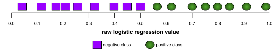
Например, на следующем рисунке показана модель классификации , которая идеально разделяет положительные классы (зеленые овалы) от отрицательных классов (фиолетовые прямоугольники). Эта нереалистично идеальная модель имеет показатель AUC, равный 1,0:
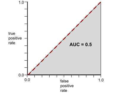
Напротив, на следующем рисунке показаны результаты для модели классификации , которая генерировала случайные результаты. Для этой модели показатель AUC равен 0,5:
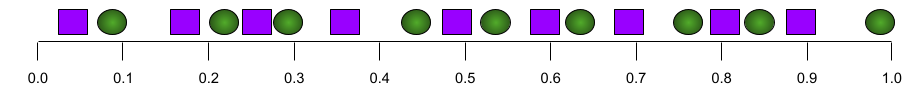
Да, у предыдущей модели показатель AUC равен 0,5, а не 0,0.
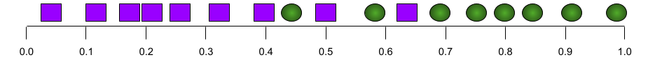
Большинство моделей находятся где-то между этими двумя крайностями. Например, следующая модель несколько разделяет положительные и отрицательные значения, и поэтому имеет AUC где-то между 0,5 и 1,0:
AUC игнорирует любые значения, которые вы задаете для порога классификации . Вместо этого AUC учитывает все возможные пороги классификации.
Нажмите на значок, чтобы узнать о взаимосвязи между AUC и ROC-кривыми.
AUC представляет собой площадь под ROC-кривой . Например, ROC-кривая для модели, которая идеально разделяет положительные и отрицательные результаты, выглядит следующим образом:
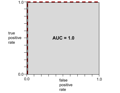
AUC — это площадь серой области на предыдущем рисунке. В этом необычном случае площадь — это просто длина серой области (1,0), умноженная на ширину серой области (1,0). Таким образом, произведение 1,0 и 1,0 дает AUC, равное ровно 1,0, что является максимально возможным значением AUC.
Напротив, ROC-кривая для модели классификации , которая вообще не может разделять классы, выглядит следующим образом. Площадь этой серой области составляет 0,5.
Типичная ROC-кривая выглядит примерно так:
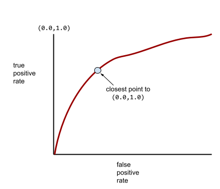
Вычисление площади под этой кривой вручную было бы трудоемким процессом, поэтому большинство значений AUC обычно рассчитываются программами.
Дополнительную информацию см. в разделе «Классификация: ROC и AUC в экспресс-курсе по машинному обучению».
дополненная реальность
Технология, которая накладывает сгенерированное компьютером изображение на реальное изображение, видимое пользователем, создавая таким образом составное изображение.
автокодировщик
Система, которая учится извлекать наиболее важную информацию из входных данных. Автокодировщики представляют собой комбинацию кодировщика и декодера . Автокодировщики используют следующий двухэтапный процесс:
- Кодировщик преобразует входные данные в (как правило) формат с потерями, имеющий промежуточную размерность.
- Декодер создает версию исходного входного сигнала с потерями, отображая формат меньшей размерности на исходный формат входного сигнала большей размерности.
Автокодировщики обучаются сквозным методом, при котором декодер пытается максимально точно восстановить исходный входной сигнал из промежуточного формата кодировщика. Поскольку промежуточный формат меньше (менее размерен), чем исходный формат, автокодировщик вынужден изучать, какая информация во входных данных является существенной, и выходные данные не будут идеально идентичны входным.
Например:
- Если входные данные представляют собой графическое изображение, то неточная копия будет похожа на исходное изображение, но несколько изменена. Возможно, неточная копия удаляет шум из исходного изображения или заполняет некоторые недостающие пиксели.
- Если входные данные представляют собой текст, автокодировщик сгенерирует новый текст, который будет имитировать (но не идентичен) исходному тексту.
См. также вариационные автокодировщики .
автоматическая оценка
Использование программного обеспечения для оценки качества результатов работы модели.
Когда выходные данные модели относительно просты, скрипт или программа могут сравнить выходные данные модели с эталонным ответом . Этот тип автоматической оценки иногда называют программной оценкой . Для программной оценки часто полезны такие метрики, как ROUGE или BLEU .
Когда результаты работы модели сложны или не имеют единственно правильного ответа , иногда автоматическую оценку выполняет отдельная программа машинного обучения, называемая авторизатором .
Сравните с человеческой оценкой .
предвзятость автоматизации
Когда человек, принимающий решения, отдает предпочтение рекомендациям автоматизированной системы принятия решений перед информацией, полученной без автоматизации, даже если автоматизированная система принятия решений допускает ошибки.
Дополнительную информацию см. в разделе «Справедливость: виды предвзятости в экспресс-курсе по машинному обучению».
AutoML
Любой автоматизированный процесс построения моделей машинного обучения . AutoML может автоматически выполнять такие задачи, как:
- Найдите наиболее подходящую модель.
- Настройте гиперпараметры .
- Подготовка данных (включая выполнение инженерии признаков ).
- Разверните полученную модель.
AutoML полезен для специалистов по обработке данных, поскольку позволяет сэкономить время и усилия при разработке конвейеров машинного обучения и повысить точность прогнозирования. Он также полезен для неспециалистов, делая сложные задачи машинного обучения более доступными для них.
Дополнительную информацию см. в разделе «Автоматизированное машинное обучение (AutoML)» в «Кратком курсе по машинному обучению».
автономный агент
Агент, который работает над достижением сложной цели, планируя, действуя и адаптируясь без постоянного вмешательства человека.
авторская оценка
Гибридный механизм оценки качества результатов работы генеративной модели ИИ , сочетающий в себе оценку человеком и автоматическую оценку . Авторефер — это модель машинного обучения, обученная на данных, созданных в результате оценки человеком . В идеале авторефер учится имитировать действия человека-оценщика.В продаже имеются готовые автоматизированные системы оценки, но лучшие из них специально оптимизированы для решения конкретной задачи.
авторегрессионная модель
Модель , которая делает вывод на основе собственных предыдущих прогнозов. Например, авторегрессивные языковые модели прогнозируют следующий токен на основе ранее предсказанных токенов. Все большие языковые модели на основе Transformer являются авторегрессивными.
В отличие от них, модели обработки изображений на основе GAN обычно не являются авторегрессивными, поскольку они генерируют изображение за один прямой проход, а не итеративно пошагово. Однако некоторые модели генерации изображений являются авторегрессивными, поскольку они генерируют изображение пошагово.
вспомогательные потери
Функция потерь — используемая совместно с основной функцией потерь модели нейронной сети — помогает ускорить обучение на ранних итерациях, когда веса инициализируются случайным образом.
Вспомогательные функции потерь переносят эффективные градиенты на более ранние слои . Это способствует сходимости во время обучения , борясь с проблемой затухания градиента .
средняя точность при k
Метрика, суммирующая производительность модели при обработке одного запроса, генерирующего ранжированные результаты, например, нумерованный список рекомендаций книг. Средняя точность в точке k — это, собственно, среднее значение точности в точке k для каждого релевантного результата. Формула для расчета средней точности в точке k выглядит следующим образом:
\[{\text{average precision at k}} = \frac{1}{n} \sum_{i=1}^n {\text{precision at k for each relevant item} } \]
где:
- \(n\) — это количество релевантных элементов в списке.
Сравните с результатами запоминания в точке k .
условие выравнивания по осям
В дереве решений условие , включающее только один признак . Например, если признаком является area , то следующее условие соответствует оси распределения:
area > 200
Сравните с косым расположением .
Б
обратное распространение
Алгоритм, реализующий градиентный спуск в нейронных сетях .
Обучение нейронной сети включает в себя множество итераций следующего двухэтапного цикла:
- В процессе прямого прохода система обрабатывает пакет примеров для получения прогнозов. Система сравнивает каждый прогноз с каждым значением метки . Разница между прогнозом и значением метки представляет собой ошибку для данного примера. Система суммирует ошибки для всех примеров, чтобы вычислить общую ошибку для текущего пакета.
- В процессе обратного распространения ошибки система уменьшает потери, корректируя веса всех нейронов во всех скрытых слоях .
Нейронные сети часто содержат множество нейронов в различных скрытых слоях. Каждый из этих нейронов вносит свой вклад в общую функцию потерь. Обратное распространение ошибки определяет, следует ли увеличивать или уменьшать веса, применяемые к конкретным нейронам.
Скорость обучения — это множитель, который регулирует степень увеличения или уменьшения каждого веса при каждом обратном проходе. Высокая скорость обучения будет увеличивать или уменьшать каждый вес сильнее, чем низкая скорость обучения.
В терминах математического анализа, обратное распространение ошибки реализует правило цепочки из математического анализа. То есть, обратное распространение ошибки вычисляет частную производную ошибки по каждому параметру.
Несколько лет назад специалистам по машинному обучению приходилось писать код для реализации обратного распространения ошибки. Современные API для машинного обучения, такие как Keras, теперь реализуют обратное распространение ошибки автоматически. Уф!
Для получения более подробной информации см. раздел «Нейронные сети в кратком курсе по машинному обучению».
упаковка
Метод обучения ансамбля , в котором каждая составляющая модель обучается на случайном подмножестве обучающих примеров, выбранных с замещением . Например, случайный лес — это набор деревьев решений, обученных с помощью метода бэггинга.
Термин bagging является сокращением от bootstrap aggregate .
Дополнительную информацию см. в разделе «Случайные леса» курса «Лесорешения».
мешок слов
Представление слов во фразе или отрывке текста независимо от порядка их следования. Например, «мешок слов» идентично представляет следующие три фразы:
- собака прыгает
- прыгает на собаку
- собака перепрыгивает
Каждое слово сопоставляется с индексом в разреженном векторе , где вектор содержит индекс для каждого слова в словаре. Например, фраза «собака прыгает» сопоставляется с вектором признаков, имеющим ненулевые значения в трех индексах, соответствующих словам «собака» , «собака» и «прыгает» . Ненулевое значение может быть любым из следующих:
- Цифра 1 обозначает наличие слова.
- Подсчет количества вхождений слова в набор. Например, если фраза "were the maroon dog is a dog with maroon fur" (бордовая собака — собака с бордовой шерстью) , то слова "maroon" и "dog" будут представлены как 2, а остальные слова — как 1.
- Какое-либо другое значение, например, логарифм количества появлений слова в мешке.
исходный уровень
Модель, используемая в качестве эталона для сравнения эффективности другой модели (как правило, более сложной). Например, модель логистической регрессии может служить хорошей базовой моделью для глубокой модели .
Для решения конкретной задачи базовый уровень помогает разработчикам моделей количественно оценить минимальную ожидаемую производительность, которую должна достичь новая модель, чтобы быть полезной.
базовая модель
Предварительно обученная модель , которая может служить отправной точкой для тонкой настройки с целью решения конкретных задач или приложений.
См. также предварительно обученную модель и базовую модель .
партия
Набор примеров, используемых в одной итерации обучения. Размер пакета определяет количество примеров в пакете.
См. раздел «Эпоха» для объяснения того, как пакет данных соотносится с эпохой.
Для получения более подробной информации см. статью «Линейная регрессия: гиперпараметры в машинном обучении».
пакетный вывод
Процесс вывода прогнозов на основе множества немаркированных примеров, разделенных на более мелкие подмножества («пакеты»).
Пакетный вывод может использовать преимущества возможностей распараллеливания, предоставляемых чипами ускорителей . То есть, несколько ускорителей могут одновременно делать прогнозы на разных пакетах немаркированных примеров, что значительно увеличивает количество выводов в секунду.
Дополнительную информацию можно найти в разделе «Системы машинного обучения в производственной среде: статический и динамический вывод» в «Кратком курсе по машинному обучению».
пакетная нормализация
Нормализация входных или выходных данных функций активации в скрытом слое . Пакетная нормализация может обеспечить следующие преимущества:
- Повысьте стабильность нейронных сетей , защитив их от выбросов в весовых коэффициентах.
- Необходимо обеспечить более высокую скорость обучения , что может ускорить тренировку.
- Уменьшите переобучение .
размер партии
Количество примеров в пакете . Например, если размер пакета равен 100, то модель обрабатывает 100 примеров за итерацию .
Ниже представлены популярные стратегии определения размера партии:
- Стохастический градиентный спуск (SGD) , в котором размер пакета равен 1.
- Полный пакет (Full batch) — это стратегия, в которой размер пакета равен количеству примеров во всем обучающем наборе данных . Например, если обучающий набор содержит миллион примеров, то размер пакета будет равен миллиону примеров. Стратегия полного пакета обычно неэффективна.
- Мини-партии, размер партии которых обычно составляет от 10 до 1000 единиц. Мини-партии, как правило, являются наиболее эффективной стратегией.
Дополнительную информацию см. ниже:
- Системы машинного обучения для производственных целей: статический и динамический вывод в кратком курсе по машинному обучению.
- Руководство по настройке глубокого обучения .
Байесовская нейронная сеть
Вероятностная нейронная сеть , учитывающая неопределенность весов и выходных данных. Стандартная модель регрессии на основе нейронной сети обычно предсказывает скалярное значение; например, стандартная модель предсказывает цену дома в 853 000. В отличие от этого, байесовская нейронная сеть предсказывает распределение значений; например, байесовская модель предсказывает цену дома в 853 000 со стандартным отклонением 67 200.
Байесовская нейронная сеть использует теорему Байеса для вычисления неопределенностей в весах и прогнозах. Байесовская нейронная сеть может быть полезна, когда важно количественно оценить неопределенность, например, в моделях, связанных с фармацевтикой. Байесовские нейронные сети также могут помочь предотвратить переобучение .
Байесовская оптимизация
Метод вероятностной регрессионной модели для оптимизации ресурсоемких целевых функций путем оптимизации аппроксимирующей функции, которая количественно оценивает неопределенность с помощью байесовского обучения. Поскольку байесовская оптимизация сама по себе очень затратна, она обычно используется для оптимизации сложных задач с небольшим количеством параметров, таких как выбор гиперпараметров .
Уравнение Беллмана
В обучении с подкреплением оптимальной Q-функции удовлетворяет следующее тождество:
\[Q(s, a) = r(s, a) + \gamma \mathbb{E}_{s'|s,a} \max_{a'} Q(s', a')\]
Алгоритмы обучения с подкреплением применяют это тождество для создания Q-обучения , используя следующее правило обновления:
\[Q(s,a) \gets Q(s,a) + \alpha \left[r(s,a) + \gamma \displaystyle\max_{\substack{a_1}} Q(s',a') - Q(s,a) \right] \]
Помимо обучения с подкреплением, уравнение Беллмана находит применение в динамическом программировании. См. статью в Википедии об уравнении Беллмана .
BERT (Bidirectional Encoder Representations from Transformers)
Архитектура модели для представления текста. Обученная модель BERT может выступать в качестве части более крупной модели для классификации текста или других задач машинного обучения.
BERT обладает следующими характеристиками:
- Использует архитектуру Transformer и, следовательно, полагается на механизм самовнимания .
- Использует кодировщик, являющийся частью трансформера. Задача кодировщика — создавать качественные текстовые представления, а не выполнять какую-либо конкретную задачу, например, классификацию.
- Является двунаправленным .
- Использует маскирование для обучения без учителя .
Варианты BERT включают в себя:
Для получения общего обзора BERT см. статью «Открытый исходный код BERT: передовое предварительное обучение для обработки естественного языка» .
bias (ethics/fairness)
1. Stereotyping, prejudice or favoritism towards some things, people, or groups over others. These biases can affect collection and interpretation of data, the design of a system, and how users interact with a system. Forms of this type of bias include:
- automation bias
- предвзятость подтверждения
- experimenter's bias
- group attribution bias
- неявная предвзятость
- in-group bias
- out-group homogeneity bias
2. Systematic error introduced by a sampling or reporting procedure. Forms of this type of bias include:
Not to be confused with the bias term in machine learning models or prediction bias .
See Fairness: Types of bias in Machine Learning Crash Course for more information.
bias (math) or bias term
An intercept or offset from an origin. Bias is a parameter in machine learning models, which is symbolized by either of the following:
- б
- w 0
For example, bias is the b in the following formula:
In a simple two-dimensional line, bias just means "y-intercept." For example, the bias of the line in the following illustration is 2.
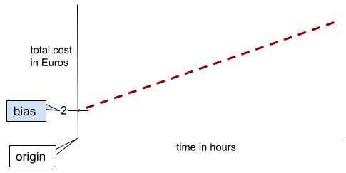
Bias exists because not all models start from the origin (0,0). For example, suppose an amusement park costs 2 Euros to enter and an additional 0.5 Euro for every hour a customer stays. Therefore, a model mapping the total cost has a bias of 2 because the lowest cost is 2 Euros.
Bias is not to be confused with bias in ethics and fairness or prediction bias .
See Linear Regression in Machine Learning Crash Course for more information.
двунаправленный
A term used to describe a system that evaluates the text that both precedes and follows a target section of text. In contrast, a unidirectional system only evaluates the text that precedes a target section of text.
For example, consider a masked language model that must determine probabilities for the word or words representing the underline in the following question:
What is the _____ with you?
A unidirectional language model would have to base its probabilities only on the context provided by the words "What", "is", and "the". In contrast, a bidirectional language model could also gain context from "with" and "you", which might help the model generate better predictions.
bidirectional language model
A language model that determines the probability that a given token is present at a given location in an excerpt of text based on the preceding and following text.
bigram
An N-gram in which N=2.
binary classification
A type of classification task that predicts one of two mutually exclusive classes:
- the positive class
- the negative class
For example, the following two machine learning models each perform binary classification:
- A model that determines whether email messages are spam (the positive class) or not spam (the negative class).
- A model that evaluates medical symptoms to determine whether a person has a particular disease (the positive class) or doesn't have that disease (the negative class).
Contrast with multi-class classification .
See also logistic regression and classification threshold .
See Classification in Machine Learning Crash Course for more information.
binary condition
In a decision tree , a condition that has only two possible outcomes, typically yes or no . For example, the following is a binary condition:
temperature >= 100
Contrast with non-binary condition .
See Types of conditions in the Decision Forests course for more information.
binning
Synonym for bucketing .
black box model
A model whose "reasoning" is impossible or difficult for humans to understand. That is, although humans can see how prompts affect responses , humans can't determine exactly how a black box model determines the response. In other words, a black box model is lacking interpretability .
Most deep models and large language models are black boxes.
BLEU (Bilingual Evaluation Understudy)
A metric between 0.0 and 1.0 for evaluating machine translations , for example, from Spanish to Japanese.
To calculate a score, BLEU typically compares an ML model's translation ( generated text ) to a human expert's translation ( reference text ). The degree to which N-grams in the generated text and reference text match determines the BLEU score.
The original paper on this metric is BLEU: a Method for Automatic Evaluation of Machine Translation .
See also BLEURT .
BLEURT (Bilingual Evaluation Understudy from Transformers)
A metric for evaluating machine translations from one language to another, particularly to and from English.
For translations to and from English, BLEURT aligns more closely to human ratings than BLEU . Unlike BLEU, BLEURT emphasizes semantic (meaning) similarities and can accommodate paraphrasing.
BLEURT relies on a pre-trained large language model ( BERT to be exact) that is then fine-tuned on text from human translators.
The original paper on this metric is BLEURT: Learning Robust Metrics for Text Generation .
Boolean Questions (BoolQ)
A dataset for evaluating an LLM's proficiency in answering yes-or-no questions. Each of the challenges in the dataset has three components:
- A query
- A passage implying the answer to the query.
- The correct answer, which is either yes or no .
Например:
- Query : Are there any nuclear power plants in Michigan?
- Passage : ...three nuclear power plants supply Michigan with about 30% of its electricity.
- Correct answer : Yes
Researchers gathered the questions from anonymized, aggregated Google Search queries and then used Wikipedia pages to ground the information.
For more information, see BoolQ: Exploring the Surprising Difficulty of Natural Yes/No Questions .
BoolQ is a component of the SuperGLUE ensemble.
BoolQ
Abbreviation for Boolean Questions .
boosting
A machine learning technique that iteratively combines a set of simple and not very accurate classification models (referred to as "weak classifiers") into a classification model with high accuracy (a "strong classifier") by upweighting the examples that the model is currently misclassifying.
See Gradient Boosted Decision Trees? in the Decision Forests course for more information.
bounding box
In an image, the ( x , y ) coordinates of a rectangle around an area of interest, such as the dog in the image below.

вещание
Expanding the shape of an operand in a matrix math operation to dimensions compatible for that operation. For example, linear algebra requires that the two operands in a matrix addition operation must have the same dimensions. Consequently, you can't add a matrix of shape (m, n) to a vector of length n. Broadcasting enables this operation by virtually expanding the vector of length n to a matrix of shape (m, n) by replicating the same values down each column.
See the following description of broadcasting in NumPy for more details.
ведро
Converting a single feature into multiple binary features called buckets or bins , typically based on a value range. The chopped feature is typically a continuous feature .
For example, instead of representing temperature as a single continuous floating-point feature, you could chop ranges of temperatures into discrete buckets, such as:
- <= 10 degrees Celsius would be the "cold" bucket.
- 11 - 24 degrees Celsius would be the "temperate" bucket.
- >= 25 degrees Celsius would be the "warm" bucket.
The model will treat every value in the same bucket identically. For example, the values 13 and 22 are both in the temperate bucket, so the model treats the two values identically.
See Numerical data: Binning in Machine Learning Crash Course for more information.
С
calibration layer
A post-prediction adjustment, typically to account for prediction bias . The adjusted predictions and probabilities should match the distribution of an observed set of labels.
candidate generation
The initial set of recommendations chosen by a recommendation system . For example, consider a bookstore that offers 100,000 titles. The candidate generation phase creates a much smaller list of suitable books for a particular user, say 500. But even 500 books is way too many to recommend to a user. Subsequent, more expensive, phases of a recommendation system (such as scoring and re-ranking ) reduce those 500 to a much smaller, more useful set of recommendations.
See Candidate generation overview in the Recommendation Systems course for more information.
candidate sampling
A training-time optimization that calculates a probability for all the positive labels, using, for example, softmax , but only for a random sample of negative labels. For instance, given an example labeled beagle and dog , candidate sampling computes the predicted probabilities and corresponding loss terms for:
- бигль
- собака
- a random subset of the remaining negative classes (for example, cat , lollipop , fence ).
The idea is that the negative classes can learn from less frequent negative reinforcement as long as positive classes always get proper positive reinforcement, and this is indeed observed empirically.
Candidate sampling is more computationally efficient than training algorithms that compute predictions for all negative classes, particularly when the number of negative classes is very large.
categorical data
Features having a specific set of possible values. For example, consider a categorical feature named traffic-light-state , which can only have one of the following three possible values:
-
red -
yellow -
green
By representing traffic-light-state as a categorical feature, a model can learn the differing impacts of red , green , and yellow on driver behavior.
Categorical features are sometimes called discrete features .
Contrast with numerical data .
See Working with categorical data in Machine Learning Crash Course for more information.
causal language model
Synonym for unidirectional language model .
See bidirectional language model to contrast different directional approaches in language modeling.
КБ
Abbreviation for CommitmentBank .
центроид
The center of a cluster as determined by a k-means or k-median algorithm. For example, if k is 3, then the k-means or k-median algorithm finds 3 centroids.
See Clustering algorithms in the Clustering course for more information.
centroid-based clustering
A category of clustering algorithms that organizes data into nonhierarchical clusters. k-means is the most widely used centroid-based clustering algorithm.
Contrast with hierarchical clustering algorithms.
See Clustering algorithms in the Clustering course for more information.
chain-of-thought prompting
A prompt engineering technique that encourages a large language model (LLM) to explain its reasoning, step by step. For example, consider the following prompt, paying particular attention to the second sentence:
How many g forces would a driver experience in a car that goes from 0 to 60 miles per hour in 7 seconds? In the answer, show all relevant calculations.
The LLM's response would likely:
- Show a sequence of physics formulas, plugging in the values 0, 60, and 7 in appropriate places.
- Explain why it chose those formulas and what the various variables mean.
Chain-of-thought prompting forces the LLM to perform all the calculations, which might lead to a more correct answer. In addition, chain-of-thought prompting enables the user to examine the LLM's steps to determine whether or not the answer makes sense.
Character N-gram F-score (ChrF)
A metric to evaluate machine translation models. Character N-gram F-score determines the degree to which N-grams in reference text overlap the N-grams in an ML model's generated text .
Character N-gram F-score is similar to metrics in the ROUGE and BLEU families, except that:
- Character N-gram F-score operates on character N-grams.
- ROUGE and BLEU operate on word N-grams or tokens .
чат
The contents of a back-and-forth dialogue with an ML system, typically a large language model . The previous interaction in a chat (what you typed and how the large language model responded) becomes the context for subsequent parts of the chat.
A chatbot is an application of a large language model.
контрольно-пропускной пункт
Data that captures the state of a model's parameters either during training or after training is completed. For example, during training, you can:
- Stop training, perhaps intentionally or perhaps as the result of certain errors.
- Capture the checkpoint.
- Later, reload the checkpoint, possibly on different hardware.
- Restart training.
Choice of Plausible Alternatives (COPA)
A dataset for evaluating how well an LLM can identify the better of two alternative answers to a premise. Each of the challenges in the dataset consists of three components:
- A premise, which is typically a statement followed by a question
- Two possible answers to the question posed in the premise, one of which is correct and the other incorrect
- Правильный ответ
Например:
- Premise: The man broke his toe. What was the CAUSE of this?
- Possible answers:
- He got a hole in his sock.
- He dropped a hammer on his foot.
- Correct answer: 2
COPA is a component of the SuperGLUE ensemble.
citation precision
A metric that answers the following question:
What percentage of the citations in an LLM's response were actually correct and supportive?
That is, what percent of the citations contain the exact facts or relevant information required to verify the claim made in an LLM's response.
For example, if an LLM response cited 10 documents, but only 7 of those citations were correct and supportive, then the citation precision would be 0.7.
citation recall
A metric that answers the following question:
What percentage of the source documents the LLM used to compose its response are actually cited in the response?
For example, if an LLM relied on 20 documents to compose its response but the response only cited 11 of them, then the citation recall would be 0.55.
сорт
A category that a label can belong to. For example:
- In a binary classification model that detects spam, the two classes might be spam and not spam .
- In a multi-class classification model that identifies dog breeds, the classes might be poodle , beagle , pug , and so on.
A classification model predicts a class. In contrast, a regression model predicts a number rather than a class.
See Classification in Machine Learning Crash Course for more information.
class-balanced dataset
A dataset containing categorical labels in which the number of instances of each category is approximately equal. For example, consider a botanical dataset whose binary label can be either native plant or nonnative plant :
- A dataset with 515 native plants and 485 nonnative plants is a class-balanced dataset.
- A dataset with 875 native plants and 125 nonnative plants is a class-imbalanced dataset .
A formal dividing line between class-balanced datasets and class-imbalanced datasets doesn't exist. The distinction only becomes important when a model trained on a highly class-imbalanced dataset can't converge. See Datasets: imbalanced datasets in Machine Learning Crash Course for details.
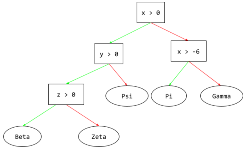
classification model
A model whose prediction is a class . For example, the following are all classification models:
- A model that predicts an input sentence's language (French? Spanish? Italian?).
- A model that predicts tree species (Maple? Oak? Baobab?).
- A model that predicts the positive or negative class for a particular medical condition.
In contrast, regression models predict numbers rather than classes.
Two common types of classification models are:
classification threshold
In a binary classification , a number between 0 and 1 that converts the raw output of a logistic regression model into a prediction of either the positive class or the negative class . Note that the classification threshold is a value that a human chooses, not a value chosen by model training.
A logistic regression model outputs a raw value between 0 and 1. Then:
- If this raw value is greater than the classification threshold, then the positive class is predicted.
- If this raw value is less than the classification threshold, then the negative class is predicted.
For example, suppose the classification threshold is 0.8. If the raw value is 0.9, then the model predicts the positive class. If the raw value is 0.7, then the model predicts the negative class.
The choice of classification threshold strongly influences the number of false positives and false negatives .
See Thresholds and the confusion matrix in Machine Learning Crash Course for more information.
классификатор
A casual term for a classification model .
class-imbalanced dataset
A dataset for a classification in which the total number of labels of each class differs significantly. For example, consider a binary classification dataset whose two labels are divided as follows:
- 1,000,000 negative labels
- 10 positive labels
The ratio of negative to positive labels is 100,000 to 1, so this is a class-imbalanced dataset.
In contrast, the following dataset is class-balanced because the ratio of negative labels to positive labels is relatively close to 1:
- 517 negative labels
- 483 positive labels
Multi-class datasets can also be class-imbalanced. For example, the following multi-class classification dataset is also class-imbalanced because one label has far more examples than the other two:
- 1,000,000 labels with class "green"
- 200 labels with class "purple"
- 350 labels with class "orange"
Training class-imbalanced datasets can present special challenges. See Imbalanced datasets in Machine Learning Crash Course for details.
See also entropy , majority class , and minority class .
обрезка
A technique for handling outliers by doing either or both of the following:
- Reducing feature values that are greater than a maximum threshold down to that maximum threshold.
- Increasing feature values that are less than a minimum threshold up to that minimum threshold.
For example, suppose that <0.5% of values for a particular feature fall outside the range 40–60. In this case, you could do the following:
- Clip all values over 60 (the maximum threshold) to be exactly 60.
- Clip all values under 40 (the minimum threshold) to be exactly 40.
Outliers can damage models, sometimes causing weights to overflow during training. Some outliers can also dramatically spoil metrics like accuracy . Clipping is a common technique to limit the damage.
Gradient clipping forces gradient values within a designated range during training.
See Numerical data: Normalization in Machine Learning Crash Course for more information.
Cloud TPU
A specialized hardware accelerator designed to speed up machine learning workloads on Google Cloud.
clustering
Grouping related examples , particularly during unsupervised learning . Once all the examples are grouped, a human can optionally supply meaning to each cluster.
Many clustering algorithms exist. For example, the k-means algorithm clusters examples based on their proximity to a centroid , as in the following diagram:

A human researcher could then review the clusters and, for example, label cluster 1 as "dwarf trees" and cluster 2 as "full-size trees."
As another example, consider a clustering algorithm based on an example's distance from a center point, illustrated as follows:

See the Clustering course for more information.
co-adaptation
An undesirable behavior in which neurons predict patterns in training data by relying almost exclusively on outputs of specific other neurons instead of relying on the network's behavior as a whole. When the patterns that cause co-adaptation are not present in validation data, then co-adaptation causes overfitting . Dropout regularization reduces co-adaptation because dropout ensures neurons cannot rely solely on specific other neurons.
коллаборативная фильтрация
Making predictions about the interests of one user based on the interests of many other users. Collaborative filtering is often used in recommendation systems .
See Collaborative filtering in the Recommendation Systems course for more information.
CommitmentBank (CB)
A dataset for evaluating an LLM's proficiency in determining whether the author of a passage believes a target clause within that passage. Each entry in the dataset contains:
- Отрывок
- A target clause within that passage
- A Boolean value indicating whether the passage's author believes the target clause
Например:
- Passage: What fun to hear Artemis laugh. She's such a serious child. I didn't know she had a sense of humor.
- Target clause: she had a sense of humor
- Boolean : True, which means the author believes the target clause
CommitmentBank is a component of the SuperGLUE ensemble.
compact model
Any small model designed to run on small devices with limited computational resources. For example, compact models can run on mobile phones, tablets, or embedded systems.
вычислить
(Noun) The computational resources used by a model or system, such as processing power, memory, and storage.
See accelerator chips .
concept drift
A shift in the relationship between features and the label. Over time, concept drift reduces a model's quality.
During training, the model learns the relationship between the features and their labels in the training set. If the labels in the training set are good proxies for the real-world, then the model should make good real world predictions. However, due to concept drift, the model's predictions tend to degrade over time.
For example, consider a binary classification model that predicts whether or not a certain car model is "fuel efficient." That is, the features could be:
- car weight
- engine compression
- тип трансмиссии
while the label is either:
- экономичный расход топлива
- not fuel efficient
However, the concept of "fuel efficient car" keeps changing. A car model labeled fuel efficient in 1994 would almost certainly be labeled not fuel efficient in 2024. A model suffering from concept drift tends to make less and less useful predictions over time.
Compare and contrast with nonstationarity .
состояние
In a decision tree , any node that performs a test. For example, the following decision tree contains two conditions: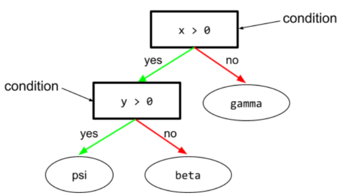
A condition is also called a split or a test.
Contrast condition with leaf .
См. также:
See Types of conditions in the Decision Forests course for more information.
конфабуляция
Synonym for hallucination .
Confabulation is probably a more technically accurate term than hallucination. However, hallucination became popular first.
конфигурация
The process of assigning the initial property values used to train a model, including:
- the model's composing layers
- the location of the data
- hyperparameters such as:
In machine learning projects, configuration can be done through a special configuration file or using configuration libraries such as the following:
предвзятость подтверждения
The tendency to search for, interpret, favor, and recall information in a way that confirms one's pre-existing beliefs or hypotheses. Machine learning developers may inadvertently collect or label data in ways that influence an outcome supporting their existing beliefs. Confirmation bias is a form of implicit bias .
Experimenter's bias is a form of confirmation bias in which an experimenter continues training models until a pre-existing hypothesis is confirmed.
матрица ошибок
An NxN table that summarizes the number of correct and incorrect predictions that a classification model made. For example, consider the following confusion matrix for a binary classification model:
| Tumor (predicted) | Non-Tumor (predicted) | |
|---|---|---|
| Tumor (ground truth) | 18 (TP) | 1 (FN) |
| Non-Tumor (ground truth) | 6 (FP) | 452 (TN) |
The preceding confusion matrix shows the following:
- Of the 19 predictions in which ground truth was Tumor, the model correctly classified 18 and incorrectly classified 1.
- Of the 458 predictions in which ground truth was Non-Tumor, the model correctly classified 452 and incorrectly classified 6.
The confusion matrix for a multi-class classification problem can help you identify patterns of mistakes. For example, consider the following confusion matrix for a 3-class multi-class classification model that categorizes three different iris types (Virginica, Versicolor, and Setosa). When the ground truth was Virginica, the confusion matrix shows that the model was far more likely to mistakenly predict Versicolor than Setosa:
| Setosa (predicted) | Versicolor (predicted) | Virginica (predicted) | |
|---|---|---|---|
| Setosa (ground truth) | 88 | 12 | 0 |
| Versicolor (ground truth) | 6 | 141 | 7 |
| Virginica (ground truth) | 2 | 27 | 109 |
As yet another example, a confusion matrix could reveal that a model trained to recognize handwritten digits tends to mistakenly predict 9 instead of 4, or mistakenly predict 1 instead of 7.
Confusion matrixes contain sufficient information to calculate a variety of performance metrics, including precision and recall .
constituency parsing
Dividing a sentence into smaller grammatical structures ("constituents"). A later part of the ML system, such as a natural language understanding model, can parse the constituents more easily than the original sentence. For example, consider the following sentence:
My friend adopted two cats.
A constituency parser can divide this sentence into the following two constituents:
- My friend is a noun phrase.
- adopted two cats is a verb phrase.
These constituents can be further subdivided into smaller constituents. For example, the verb phrase
adopted two cats
could be further subdivided into:
- adopted is a verb.
- two cats is another noun phrase.
contextualized language embedding
An embedding that comes close to "understanding" words and phrases in ways that fluent human speakers can. Contextualized language embeddings can understand complex syntax, semantics, and context.
For example, consider embeddings of the English word cow . Older embeddings such as word2vec can represent English words such that the distance in the embedding space from cow to bull is similar to the distance from ewe (female sheep) to ram (male sheep) or from female to male . Contextualized language embeddings can go a step further by recognizing that English speakers sometimes casually use the word cow to mean either cow or bull.
контекстное окно
The number of tokens a model can process in a given prompt . The larger the context window, the more information the model can use to provide coherent and consistent responses to the prompt.
continuous feature
A floating-point feature with an infinite range of possible values, such as temperature or weight.
Contrast with discrete feature .
выборочная выборка по удобству
Using a dataset not gathered scientifically in order to run quick experiments. Later on, it's essential to switch to a scientifically gathered dataset.
конвергенция
A state reached when loss values change very little or not at all with each iteration . For example, the following loss curve suggests convergence at around 700 iterations:
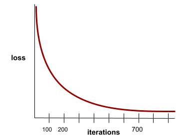
A model converges when additional training won't improve the model.
In deep learning , loss values sometimes stay constant or nearly so for many iterations before finally descending. During a long period of constant loss values, you may temporarily get a false sense of convergence.
See also early stopping .
See Model convergence and loss curves in Machine Learning Crash Course for more information.
conversational coding
An iterative dialog between you and a generative AI model for the purpose of creating software. You issue a prompt describing some software. Then, the model uses that description to generate code. Then, you issue a new prompt to address the flaws in the previous prompt or in the generated code, and the model generates updated code. You two keep going back and forth until the generated software is good enough.
Conversation coding is essentially the original meaning of vibe coding .
Contrast with specificational coding .
convex function
A function in which the region above the graph of the function is a convex set . The prototypical convex function is shaped something like the letter U . For example, the following are all convex functions:
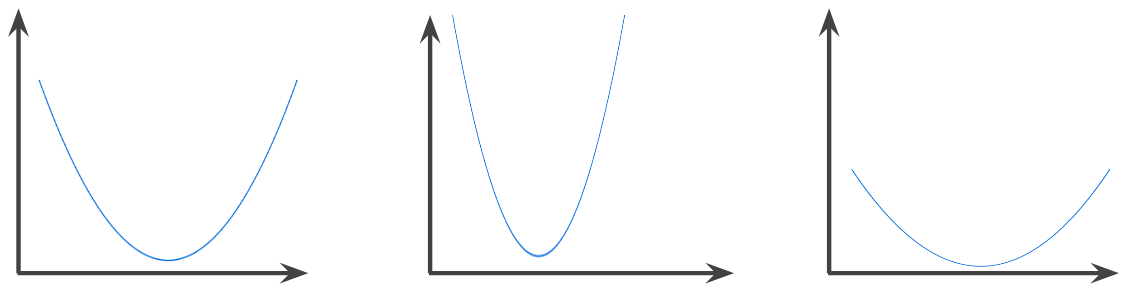
In contrast, the following function is not convex. Notice how the region above the graph is not a convex set:

A strictly convex function has exactly one local minimum point, which is also the global minimum point. The classic U-shaped functions are strictly convex functions. However, some convex functions (for example, straight lines) are not U-shaped.
See Convergence and convex functions in Machine Learning Crash Course for more information.
выпуклая оптимизация
The process of using mathematical techniques such as gradient descent to find the minimum of a convex function . A great deal of research in machine learning has focused on formulating various problems as convex optimization problems and in solving those problems more efficiently.
For complete details, see Boyd and Vandenberghe, Convex Optimization .
convex set
A subset of Euclidean space such that a line drawn between any two points in the subset remains completely within the subset. For instance, the following two shapes are convex sets:
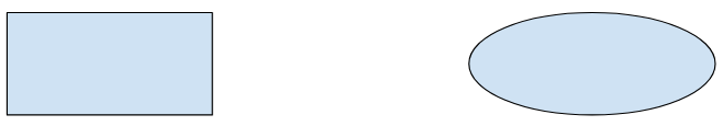
In contrast, the following two shapes are not convex sets:

свертка
In mathematics, casually speaking, a mixture of two functions. In machine learning, a convolution mixes the convolutional filter and the input matrix in order to train weights .
The term "convolution" in machine learning is often a shorthand way of referring to either convolutional operation or convolutional layer .
Without convolutions, a machine learning algorithm would have to learn a separate weight for every cell in a large tensor . For example, a machine learning algorithm training on 2K x 2K images would be forced to find 4M separate weights. Thanks to convolutions, a machine learning algorithm only has to find weights for every cell in the convolutional filter , dramatically reducing the memory needed to train the model. When the convolutional filter is applied, it is simply replicated across cells such that each is multiplied by the filter.
convolutional filter
One of the two actors in a convolutional operation . (The other actor is a slice of an input matrix.) A convolutional filter is a matrix having the same rank as the input matrix, but a smaller shape. For example, given a 28x28 input matrix, the filter could be any 2D matrix smaller than 28x28.
In photographic manipulation, all the cells in a convolutional filter are typically set to a constant pattern of ones and zeroes. In machine learning, convolutional filters are typically seeded with random numbers and then the network trains the ideal values.
сверточный слой
A layer of a deep neural network in which a convolutional filter passes along an input matrix. For example, consider the following 3x3 convolutional filter :
![A 3x3 matrix with the following values: [[0,1,0], [1,0,1], [0,1,0]]](https://developers.google.com/static/machine-learning/glossary/images/ConvolutionalFilter33.svg?authuser=1&hl=ru)
The following animation shows a convolutional layer consisting of 9 convolutional operations involving the 5x5 input matrix. Notice that each convolutional operation works on a different 3x3 slice of the input matrix. The resulting 3x3 matrix (on the right) consists of the results of the 9 convolutional operations:
![An animation showing two matrixes. The first matrix is the 5x5
matrix: [[128,97,53,201,198], [35,22,25,200,195],
[37,24,28,197,182], [33,28,92,195,179], [31,40,100,192,177]].
The second matrix is the 3x3 matrix:
[[181,303,618], [115,338,605], [169,351,560]].
The second matrix is calculated by applying the convolutional
filter [[0, 1, 0], [1, 0, 1], [0, 1, 0]] across
different 3x3 subsets of the 5x5 matrix.](https://developers.google.com/static/machine-learning/glossary/images/AnimatedConvolution.gif?authuser=1&hl=ru)
сверточная нейронная сеть
A neural network in which at least one layer is a convolutional layer . A typical convolutional neural network consists of some combination of the following layers:
Convolutional neural networks have had great success in certain kinds of problems, such as image recognition.
convolutional operation
The following two-step mathematical operation:
- Element-wise multiplication of the convolutional filter and a slice of an input matrix. (The slice of the input matrix has the same rank and size as the convolutional filter.)
- Summation of all the values in the resulting product matrix.
For example, consider the following 5x5 input matrix:
![The 5x5 matrix: [[128,97,53,201,198], [35,22,25,200,195],
[37,24,28,197,182], [33,28,92,195,179], [31,40,100,192,177]].](https://developers.google.com/static/machine-learning/glossary/images/ConvolutionalLayerInputMatrix.svg?authuser=1&hl=ru)
Now imagine the following 2x2 convolutional filter:
![The 2x2 matrix: [[1, 0], [0, 1]]](https://developers.google.com/static/machine-learning/glossary/images/ConvolutionalLayerFilter.svg?authuser=1&hl=ru)
Each convolutional operation involves a single 2x2 slice of the input matrix. For example, suppose we use the 2x2 slice at the top-left of the input matrix. So, the convolution operation on this slice looks as follows:
![Applying the convolutional filter [[1, 0], [0, 1]] to the top-left
2x2 section of the input matrix, which is [[128,97], [35,22]].
The convolutional filter leaves the 128 and 22 intact, but zeroes
out the 97 and 35. Consequently, the convolution operation yields
the value 150 (128+22).](https://developers.google.com/static/machine-learning/glossary/images/ConvolutionalLayerOperation.svg?authuser=1&hl=ru)
A convolutional layer consists of a series of convolutional operations, each acting on a different slice of the input matrix.
КОПА
Abbreviation for Choice of Plausible Alternatives .
расходы
Synonym for loss .
co-training
A semi-supervised learning approach particularly useful when all of the following conditions are true:
- The ratio of unlabeled examples to labeled examples in the dataset is high.
- This is a classification problem ( binary or multi-class ).
- The dataset contains two different sets of predictive features that are independent of each other and complementary.
Co-training essentially amplifies independent signals into a stronger signal. For example, consider a classification model that categorizes individual used cars as either Good or Bad . One set of predictive features might focus on aggregate characteristics such as the year, make, and model of the car; another set of predictive features might focus on the previous owner's driving record and the car's maintenance history.
The seminal paper on co-training is Combining Labeled and Unlabeled Data with Co-Training by Blum and Mitchell.
counterfactual fairness
A fairness metric that checks whether a classification model produces the same result for one individual as it does for another individual who is identical to the first, except with respect to one or more sensitive attributes . Evaluating a classification model for counterfactual fairness is one method for surfacing potential sources of bias in a model.
See either of the following for more information:
- Fairness: Counterfactual fairness in Machine Learning Crash Course.
- When Worlds Collide: Integrating Different Counterfactual Assumptions in Fairness
coverage bias
See selection bias .
crash blossom
A sentence or phrase with an ambiguous meaning. Crash blossoms present a significant problem in natural language understanding . For example, the headline Red Tape Holds Up Skyscraper is a crash blossom because an NLU model could interpret the headline literally or figuratively.
критик
Synonym for Deep Q-Network .
перекрестная энтропия
A generalization of Log Loss to multi-class classification problems . Cross-entropy quantifies the difference between two probability distributions. See also perplexity .
cross-validation
A mechanism for estimating how well a model would generalize to new data by testing the model against one or more non-overlapping data subsets withheld from the training set .
cumulative distribution function (CDF)
A function that defines the frequency of samples less than or equal to a target value. For example, consider a normal distribution of continuous values. A CDF tells you that approximately 50% of samples should be less than or equal to the mean and that approximately 84% of samples should be less than or equal to one standard deviation above the mean.
Д
анализ данных
Obtaining an understanding of data by considering samples, measurement, and visualization. Data analysis can be particularly useful when a dataset is first received, before one builds the first model . It is also crucial in understanding experiments and debugging problems with the system.
data augmentation
Artificially boosting the range and number of training examples by transforming existing examples to create additional examples. For example, suppose images are one of your features , but your dataset doesn't contain enough image examples for the model to learn useful associations. Ideally, you'd add enough labeled images to your dataset to enable your model to train properly. If that's not possible, data augmentation can rotate, stretch, and reflect each image to produce many variants of the original picture, possibly yielding enough labeled data to enable excellent training.
DataFrame
A popular pandas data type for representing datasets in memory.
A DataFrame is analogous to a table or a spreadsheet. Each column of a DataFrame has a name (a header), and each row is identified by a unique number.
Each column in a DataFrame is structured like a 2D array, except that each column can be assigned its own data type.
See also the official pandas.DataFrame reference page .
data parallelism
A way of scaling training or inference that replicates an entire model onto multiple devices and then passes a subset of the input data to each device. Data parallelism can enable training and inference on very large batch sizes ; however, data parallelism requires that the model be small enough to fit on all devices.
Data parallelism typically speeds training and inference.
See also model parallelism .
Dataset API (tf.data)
A high-level TensorFlow API for reading data and transforming it into a form that a machine learning algorithm requires. A tf.data.Dataset object represents a sequence of elements, in which each element contains one or more Tensors . A tf.data.Iterator object provides access to the elements of a Dataset .
data set or dataset
A collection of raw data, commonly (but not exclusively) organized in one of the following formats:
- a spreadsheet
- a file in CSV (comma-separated values) format
decision boundary
The separator between classes learned by a model in a binary class or multi-class classification problems . For example, in the following image representing a binary classification problem, the decision boundary is the frontier between the orange class and the blue class:

decision forest
A model created from multiple decision trees . A decision forest makes a prediction by aggregating the predictions of its decision trees. Popular types of decision forests include random forests and gradient boosted trees .
See the Decision Forests section in the Decision Forests course for more information.
decision threshold
Synonym for classification threshold .
дерево решений
A supervised learning model composed of a set of conditions and leaves organized hierarchically. For example, the following is a decision tree:
декодер
In general, any ML system that converts from a processed, dense, or internal representation to a more raw, sparse, or external representation.
Decoders are often a component of a larger model, where they are frequently paired with an encoder .
In sequence-to-sequence tasks , a decoder starts with the internal state generated by the encoder to predict the next sequence.
Refer to Transformer for the definition of a decoder within the Transformer architecture.
See Large language models in Machine Learning Crash Course for more information.
deep model
A neural network containing more than one hidden layer .
A deep model is also called a deep neural network .
Contrast with wide model .
deep neural network
Synonym for deep model .
Deep Q-Network (DQN)
In Q-learning , a deep neural network that predicts Q-functions .
Critic is a synonym for Deep Q-Network.
demographic parity
A fairness metric that is satisfied if the results of a model's classification are not dependent on a given sensitive attribute .
For example, if both Lilliputians and Brobdingnagians apply to Glubbdubdrib University, demographic parity is achieved if the percentage of Lilliputians admitted is the same as the percentage of Brobdingnagians admitted, irrespective of whether one group is on average more qualified than the other.
Contrast with equalized odds and equality of opportunity , which permit classification results in aggregate to depend on sensitive attributes, but don't permit classification results for certain specified ground truth labels to depend on sensitive attributes. See "Attacking discrimination with smarter machine learning" for a visualization exploring the tradeoffs when optimizing for demographic parity.
See Fairness: demographic parity in Machine Learning Crash Course for more information.
denoising
A common approach to self-supervised learning in which:
Denoising enables learning from unlabeled examples . The original dataset serves as the target or label and the noisy data as the input.
Some masked language models use denoising as follows:
- Noise is artificially added to an unlabeled sentence by masking some of the tokens.
- The model tries to predict the original tokens.
dense feature
A feature in which most or all values are nonzero, typically a Tensor of floating-point values. For example, the following 10-element Tensor is dense because 9 of its values are nonzero:
| 8 | 3 | 7 | 5 | 2 | 4 | 0 | 4 | 9 | 6 |
Contrast with sparse feature .
dense layer
Synonym for fully connected layer .
глубина
The sum of the following in a neural network :
- the number of hidden layers
- the number of output layers , which is typically 1
- the number of any embedding layers
For example, a neural network with five hidden layers and one output layer has a depth of 6.
Notice that the input layer doesn't influence depth.
depthwise separable convolutional neural network (sepCNN)
A convolutional neural network architecture based on Inception , but where Inception modules are replaced with depthwise separable convolutions. Also known as Xception.
A depthwise separable convolution (also abbreviated as separable convolution) factors a standard 3D convolution into two separate convolution operations that are more computationally efficient: first, a depthwise convolution, with a depth of 1 (n ✕ n ✕ 1), and then second, a pointwise convolution, with length and width of 1 (1 ✕ 1 ✕ n).
To learn more, see Xception: Deep Learning with Depthwise Separable Convolutions .
derived label
Synonym for proxy label .
детерминированный
A system that always returns the same output for a given input. For example, the ReLU function is deterministic because:
- When the input is negative, the output is always 0.
- When the input is nonnegative, the output always equals the input.
By contrast, a function that returns a random number each time it is called is nondeterministic .
Deterministic systems are generally much easier to test than nondeterministic systems.
LLMs are usually nondeterministic; that is, the LLM's response to the same prompt often differs.
устройство
An overloaded term with the following two possible definitions:
- A category of hardware that can run a TensorFlow session, including CPUs, GPUs, and TPUs .
- When training an ML model on accelerator chips (GPUs or TPUs), the part of the system that actually manipulates tensors and embeddings . The device runs on accelerator chips. In contrast, the host typically runs on a CPU.
differential privacy
In machine learning, an anonymization approach to protect any sensitive data (for example, an individual's personal information) included in a model's training set from being exposed. This approach ensures that the model doesn't learn or remember much about a specific individual. This is accomplished by sampling and adding noise during model training to obscure individual data points, mitigating the risk of exposing sensitive training data.
Differential privacy is also used outside of machine learning. For example, data scientists sometimes use differential privacy to protect individual privacy when computing product usage statistics for different demographics.
dimension reduction
Decreasing the number of dimensions used to represent a particular feature in a feature vector, typically by converting to an embedding vector .
размеры
Overloaded term having any of the following definitions:
The number of levels of coordinates in a Tensor . For example:
- A scalar has zero dimensions; for example,
["Hello"]. - A vector has one dimension; for example,
[3, 5, 7, 11]. - A matrix has two dimensions; for example,
[[2, 4, 18], [5, 7, 14]]. You can uniquely specify a particular cell in a one-dimensional vector with one coordinate; you need two coordinates to uniquely specify a particular cell in a two-dimensional matrix.
- A scalar has zero dimensions; for example,
The number of entries in a feature vector .
The number of elements in an embedding layer .
direct prompting
Synonym for zero-shot prompting .
discrete feature
A feature with a finite set of possible values. For example, a feature whose values may only be animal , vegetable , or mineral is a discrete (or categorical) feature.
Contrast with continuous feature .
discriminative model
A model that predicts labels from a set of one or more features . More formally, discriminative models define the conditional probability of an output given the features and weights ; that is:
p(output | features, weights)
For example, a model that predicts whether an email is spam from features and weights is a discriminative model.
The vast majority of supervised learning models, including classification and regression models, are discriminative models.
Contrast with generative model .
дискриминатор
A system that determines whether examples are real or fake.
Alternatively, the subsystem within a generative adversarial network that determines whether the examples created by the generator are real or fake.
See The discriminator in the GAN course for more information.
disparate impact
Making decisions about people that impact different population subgroups disproportionately. This usually refers to situations where an algorithmic decision-making process harms or benefits some subgroups more than others.
For example, suppose an algorithm that determines a Lilliputian's eligibility for a miniature-home loan is more likely to classify them as "ineligible" if their mailing address contains a certain postal code. If Big-Endian Lilliputians are more likely to have mailing addresses with this postal code than Little-Endian Lilliputians, then this algorithm may result in disparate impact.
Contrast with disparate treatment , which focuses on disparities that result when subgroup characteristics are explicit inputs to an algorithmic decision-making process.
disparate treatment
Factoring subjects' sensitive attributes into an algorithmic decision-making process such that different subgroups of people are treated differently.
For example, consider an algorithm that determines Lilliputians' eligibility for a miniature-home loan based on the data they provide in their loan application. If the algorithm uses a Lilliputian's affiliation as Big-Endian or Little-Endian as an input, it is enacting disparate treatment along that dimension.
Contrast with disparate impact , which focuses on disparities in the societal impacts of algorithmic decisions on subgroups, irrespective of whether those subgroups are inputs to the model.
дистилляция
The process of reducing the size of one model (known as the teacher ) into a smaller model (known as the student ) that emulates the original model's predictions as faithfully as possible. Distillation is useful because the smaller model has two key benefits over the larger model (the teacher):
- Faster inference time
- Reduced memory and energy usage
However, the student's predictions are typically not as good as the teacher's predictions.
Distillation trains the student model to minimize a loss function based on the difference between the outputs of the predictions of the student and teacher models.
Compare and contrast distillation with the following terms:
See LLMs: Fine-tuning, distillation, and prompt engineering in Machine Learning Crash Course for more information.
распределение
The frequency and range of different values for a given feature or label . A distribution captures how likely a particular value is.
The following image shows histograms of two different distributions:
- On the left, a power law distribution of wealth versus the number of people possessing that wealth.
- On the right, a normal distribution of height versus the number of people possessing that height.
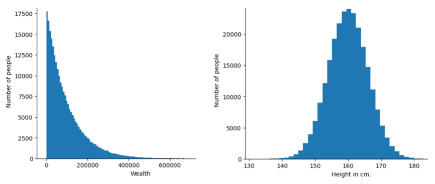
Understanding each feature and label's distribution can help you determine how to normalize values and detect outliers .
The phrase out of distribution refers to a value that doesn't appear in the dataset or is very rare. For example, an image of the planet Saturn would be considered out of distribution for a dataset consisting of cat images.
divisive clustering
See hierarchical clustering .
downsampling
Overloaded term that can mean either of the following:
- Reducing the amount of information in a feature in order to train a model more efficiently. For example, before training an image recognition model, downsampling high-resolution images to a lower-resolution format.
- Training on a disproportionately low percentage of over-represented class examples in order to improve model training on under-represented classes. For example, in a class-imbalanced dataset , models tend to learn a lot about the majority class and not enough about the minority class . Downsampling helps balance the amount of training on the majority and minority classes.
See Datasets: Imbalanced datasets in Machine Learning Crash Course for more information.
DQN
Abbreviation for Deep Q-Network .
dropout regularization
A form of regularization useful in training neural networks . Dropout regularization removes a random selection of a fixed number of the units in a network layer for a single gradient step. The more units dropped out, the stronger the regularization. This is analogous to training the network to emulate an exponentially large ensemble of smaller networks. For full details, see Dropout: A Simple Way to Prevent Neural Networks from Overfitting .
динамический
Something done frequently or continuously. The terms dynamic and online are synonyms in machine learning. The following are common uses of dynamic and online in machine learning:
- A dynamic model (or online model ) is a model that is retrained frequently or continuously.
- Dynamic training (or online training ) is the process of training frequently or continuously.
- Dynamic inference (or online inference ) is the process of generating predictions on demand.
dynamic model
A model that is frequently (maybe even continuously) retrained. A dynamic model is a "lifelong learner" that constantly adapts to evolving data. A dynamic model is also known as an online model .
Contrast with static model .
Е
eager execution
A TensorFlow programming environment in which operations run immediately. In contrast, operations called in graph execution don't run until they are explicitly evaluated. Eager execution is an imperative interface , much like the code in most programming languages. Eager execution programs are generally far easier to debug than graph execution programs.
early stopping
A method for regularization that involves ending training before training loss finishes decreasing. In early stopping, you intentionally stop training the model when the loss on a validation dataset starts to increase; that is, when generalization performance worsens.
Contrast with early exit .
earth mover's distance (EMD)
A measure of the relative similarity of two distributions . The lower the earth mover's distance, the more similar the distributions.
edit distance
A measurement of how similar two text strings are to each other. In machine learning, edit distance is useful for the following reasons:
- Edit distance is easy to compute.
- Edit distance can compare two strings known to be similar to each other.
- Edit distance can determine the degree to which different strings are similar to a given string.
Several definitions of edit distance exist, each using different string operations. See Levenshtein distance for an example.
Einsum notation
An efficient notation for describing how two tensors are to be combined. The tensors are combined by multiplying the elements of one tensor by the elements of the other tensor and then summing the products. Einsum notation uses symbols to identify the axes of each tensor, and those same symbols are rearranged to specify the shape of the new resulting tensor.
NumPy provides a common Einsum implementation.
embedding layer
A special hidden layer that trains on a high-dimensional categorical feature to gradually learn a lower dimension embedding vector. An embedding layer enables a neural network to train far more efficiently than training just on the high-dimensional categorical feature.
For example, Earth currently supports about 73,000 tree species. Suppose tree species is a feature in your model, so your model's input layer includes a one-hot vector 73,000 elements long. For example, perhaps baobab would be represented something like this:
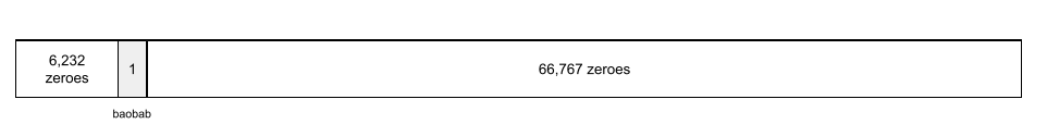
A 73,000-element array is very long. If you don't add an embedding layer to the model, training is going to be very time consuming due to multiplying 72,999 zeros. Perhaps you pick the embedding layer to consist of 12 dimensions. Consequently, the embedding layer will gradually learn a new embedding vector for each tree species.
In certain situations, hashing is a reasonable alternative to an embedding layer.
See Embeddings in Machine Learning Crash Course for more information.
embedding space
The d-dimensional vector space that features from a higher-dimensional vector space are mapped to. Embedding space is trained to capture structure that is meaningful for the intended application.
The dot product of two embeddings is a measure of their similarity.
embedding vector
Broadly speaking, an array of floating-point numbers taken from any hidden layer that describe the inputs to that hidden layer. Often, an embedding vector is the array of floating-point numbers trained in an embedding layer. For example, suppose an embedding layer must learn an embedding vector for each of the 73,000 tree species on Earth. Perhaps the following array is the embedding vector for a baobab tree:
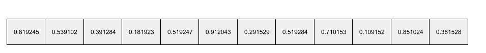
An embedding vector is not a bunch of random numbers. An embedding layer determines these values through training, similar to the way a neural network learns other weights during training. Each element of the array is a rating along some characteristic of a tree species. Which element represents which tree species' characteristic? That's very hard for humans to determine.
The mathematically remarkable part of an embedding vector is that similar items have similar sets of floating-point numbers. For example, similar tree species have a more similar set of floating-point numbers than dissimilar tree species. Redwoods and sequoias are related tree species, so they'll have a more similar set of floating-pointing numbers than redwoods and coconut palms. The numbers in the embedding vector will change each time you retrain the model, even if you retrain the model with identical input.
emergent behavior
An LLM's ability to generate responses for prompts that it was not explicitly trained on.
empirical cumulative distribution function (eCDF or EDF)
A cumulative distribution function based on empirical measurements from a real dataset. The value of the function at any point along the x-axis is the fraction of observations in the dataset that are less than or equal to the specified value.
empirical risk minimization (ERM)
Choosing the function that minimizes loss on the training set. Contrast with structural risk minimization .
кодировщик
In general, any ML system that converts from a raw, sparse, or external representation into a more processed, denser, or more internal representation.
Encoders are often a component of a larger model, where they are frequently paired with a decoder . Some Transformers pair encoders with decoders, though other Transformers use only the encoder or only the decoder.
Some systems use the encoder's output as the input to a classification or regression network.
In sequence-to-sequence tasks , an encoder takes an input sequence and returns an internal state (a vector). Then, the decoder uses that internal state to predict the next sequence.
Refer to Transformer for the definition of an encoder in the Transformer architecture.
See LLMs: What's a large language model in Machine Learning Crash Course for more information.
конечные точки
A network-addressable location (typically a URL) where a service can be reached.
ансамбль
A collection of models trained independently whose predictions are averaged or aggregated. In many cases, an ensemble produces better predictions than a single model. For example, a random forest is an ensemble built from multiple decision trees . Note that not all decision forests are ensembles.
See Random Forest in Machine Learning Crash Course for more information.
энтропия
In information theory , a description of how unpredictable a probability distribution is. Alternatively, entropy is also defined as how much information each example contains. A distribution has the highest possible entropy when all values of a random variable are equally likely.
The entropy of a set with two possible values "0" and "1" (for example, the labels in a binary classification problem) has the following formula:
H = -p log p - q log q = -p log p - (1-p) * log (1-p)
где:
- H is the entropy.
- p is the fraction of "1" examples.
- q is the fraction of "0" examples. Note that q = (1 - p)
- log is generally log 2 . In this case, the entropy unit is a bit.
For example, suppose the following:
- 100 examples contain the value "1"
- 300 examples contain the value "0"
Therefore, the entropy value is:
- p = 0.25
- q = 0.75
- H = (-0.25)log 2 (0.25) - (0.75)log 2 (0.75) = 0.81 bits per example
A set that is perfectly balanced (for example, 200 "0"s and 200 "1"s) would have an entropy of 1.0 bit per example. As a set becomes more imbalanced , its entropy moves towards 0.0.
In decision trees , entropy helps formulate information gain to help the splitter select the conditions during the growth of a classification decision tree.
Compare entropy with:
- gini impurity
- cross-entropy loss function
Entropy is often called Shannon's entropy .
See Exact splitter for binary classification with numerical features in the Decision Forests course for more information.
среда
In reinforcement learning, the world that contains the agent and allows the agent to observe that world's state . For example, the represented world can be a game like chess, or a physical world like a maze. When the agent applies an action to the environment, then the environment transitions between states.
environment grounding
The raw data that flows back to the agent during the feedback stage of the agentic loop . For example, environment grounding for an agent might include error logs or the HTML of a newly created web page.
эпизод
In reinforcement learning, each of the repeated attempts by the agent to learn an environment .
эпизодическая память
In LLMs, information learned after training. In contrast, semantic memory is information learned during training. Episodic memory can be temporary (for example, lasting only within the current chatbot session) or more permanent (for example, persisting for each session the user invokes).
See also procedural memory .
эпоха
A full training pass over the entire training set such that each example has been processed once.
An epoch represents N / batch size training iterations , where N is the total number of examples.
For instance, suppose the following:
- The dataset consists of 1,000 examples.
- The batch size is 50 examples.
Therefore, a single epoch requires 20 iterations:
1 epoch = (N/batch size) = (1,000 / 50) = 20 iterations
See Linear regression: Hyperparameters in Machine Learning Crash Course for more information.
epsilon greedy policy
In reinforcement learning, a policy that either follows a random policy with epsilon probability or a greedy policy otherwise. For example, if epsilon is 0.9, then the policy follows a random policy 90% of the time and a greedy policy 10% of the time.
Over successive episodes, the algorithm reduces epsilon's value in order to shift from following a random policy to following a greedy policy. By shifting the policy, the agent first randomly explores the environment and then greedily exploits the results of random exploration.
equality of opportunity
A fairness metric to assess whether a model is predicting the desirable outcome equally well for all values of a sensitive attribute . In other words, if the desirable outcome for a model is the positive class , the goal would be to have the true positive rate be the same for all groups.
Equality of opportunity is related to equalized odds , which requires that both the true positive rates and false positive rates are the same for all groups.
Suppose Glubbdubdrib University admits both Lilliputians and Brobdingnagians to a rigorous mathematics program. Lilliputians' secondary schools offer a robust curriculum of math classes, and the vast majority of students are qualified for the university program. Brobdingnagians' secondary schools don't offer math classes at all, and as a result, far fewer of their students are qualified. Equality of opportunity is satisfied for the preferred label of "admitted" with respect to nationality (Lilliputian or Brobdingnagian) if qualified students are equally likely to be admitted irrespective of whether they're a Lilliputian or a Brobdingnagian.
For example, suppose 100 Lilliputians and 100 Brobdingnagians apply to Glubbdubdrib University, and admissions decisions are made as follows:
Table 1. Lilliputian applicants (90% are qualified)
| Квалифицированный | Неквалифицированный | |
|---|---|---|
| Допущенный | 45 | 3 |
| Отклоненный | 45 | 7 |
| Общий | 90 | 10 |
| Percentage of qualified students admitted: 45/90 = 50% Percentage of unqualified students rejected: 7/10 = 70% Total percentage of Lilliputian students admitted: (45+3)/100 = 48% | ||
Table 2. Brobdingnagian applicants (10% are qualified):
| Квалифицированный | Неквалифицированный | |
|---|---|---|
| Допущенный | 5 | 9 |
| Отклоненный | 5 | 81 |
| Общий | 10 | 90 |
| Percentage of qualified students admitted: 5/10 = 50% Percentage of unqualified students rejected: 81/90 = 90% Total percentage of Brobdingnagian students admitted: (5+9)/100 = 14% | ||
The preceding examples satisfy equality of opportunity for acceptance of qualified students because qualified Lilliputians and Brobdingnagians both have a 50% chance of being admitted.
While equality of opportunity is satisfied, the following two fairness metrics are not satisfied:
- demographic parity : Lilliputians and Brobdingnagians are admitted to the university at different rates; 48% of Lilliputians students are admitted, but only 14% of Brobdingnagian students are admitted.
- equalized odds : While qualified Lilliputian and Brobdingnagian students both have the same chance of being admitted, the additional constraint that unqualified Lilliputians and Brobdingnagians both have the same chance of being rejected is not satisfied. Unqualified Lilliputians have a 70% rejection rate, whereas unqualified Brobdingnagians have a 90% rejection rate.
See Fairness: Equality of opportunity in Machine Learning Crash Course for more information.
equalized odds
A fairness metric to assess whether a model is predicting outcomes equally well for all values of a sensitive attribute with respect to both the positive class and negative class —not just one class or the other exclusively. In other words, both the true positive rate and false negative rate should be the same for all groups.
Equalized odds is related to equality of opportunity , which only focuses on error rates for a single class (positive or negative).
For example, suppose Glubbdubdrib University admits both Lilliputians and Brobdingnagians to a rigorous mathematics program. Lilliputians' secondary schools offer a robust curriculum of math classes, and the vast majority of students are qualified for the university program. Brobdingnagians' secondary schools don't offer math classes at all, and as a result, far fewer of their students are qualified. Equalized odds is satisfied provided that no matter whether an applicant is a Lilliputian or a Brobdingnagian, if they are qualified, they are equally as likely to get admitted to the program, and if they are not qualified, they are equally as likely to get rejected.
Suppose 100 Lilliputians and 100 Brobdingnagians apply to Glubbdubdrib University, and admissions decisions are made as follows:
Table 3. Lilliputian applicants (90% are qualified)
| Квалифицированный | Неквалифицированный | |
|---|---|---|
| Допущенный | 45 | 2 |
| Отклоненный | 45 | 8 |
| Общий | 90 | 10 |
| Percentage of qualified students admitted: 45/90 = 50% Percentage of unqualified students rejected: 8/10 = 80% Total percentage of Lilliputian students admitted: (45+2)/100 = 47% | ||
Table 4. Brobdingnagian applicants (10% are qualified):
| Квалифицированный | Неквалифицированный | |
|---|---|---|
| Допущенный | 5 | 18 |
| Отклоненный | 5 | 72 |
| Общий | 10 | 90 |
| Percentage of qualified students admitted: 5/10 = 50% Percentage of unqualified students rejected: 72/90 = 80% Total percentage of Brobdingnagian students admitted: (5+18)/100 = 23% | ||
Equalized odds is satisfied because qualified Lilliputian and Brobdingnagian students both have a 50% chance of being admitted, and unqualified Lilliputian and Brobdingnagian have an 80% chance of being rejected.
Equalized odds is formally defined in "Equality of Opportunity in Supervised Learning" as follows: "predictor Ŷ satisfies equalized odds with respect to protected attribute A and outcome Y if Ŷ and A are independent, conditional on Y."
Estimator
A deprecated TensorFlow API. Use tf.keras instead of Estimators.
оценки
Primarily used as an abbreviation for LLM evaluations . More broadly, evals is an abbreviation for any form of evaluation .
оценка
The process of measuring a model's quality or comparing different models against each other.
To evaluate a supervised machine learning model, you typically judge it against a validation set and a test set . Evaluating a LLM typically involves broader quality and safety assessments.
evaluator agent
An agent that assesses another agent's results before those results are finalized. You can imagine one agent as manufacturing a product and a separate agent—the evaluator agent—testing that product before it is released.
Critic is a synonym for evaluator agent.
точное совпадение
An all-or-nothing metric in which the model's output either matches ground truth or the reference text exactly or it doesn't. For example, if ground truth is orange , the only model output that satisfies exact match is orange .
Exact match can also evaluate models whose output is a sequence (a ranked list of items). In general, exact match requires the generated ranked list to exactly match ground truth; that is, each item in both lists must be in the same order. That said, if ground truth consists of multiple correct sequences, then exact match only requires model's output matches one of the correct sequences.
пример
The values of one row of features and possibly a label . Examples in supervised learning fall into two general categories:
- A labeled example consists of one or more features and a label. Labeled examples are used during training.
- An unlabeled example consists of one or more features but no label. Unlabeled examples are used during inference.
For instance, suppose you are training a model to determine the influence of weather conditions on student test scores. Here are three labeled examples:
| Функции | Этикетка | ||
|---|---|---|---|
| Температура | Влажность | Давление | Test score |
| 15 | 47 | 998 | Хороший |
| 19 | 34 | 1020 | Отличный |
| 18 | 92 | 1012 | Бедный |
Here are three unlabeled examples:
| Температура | Влажность | Давление | |
|---|---|---|---|
| 12 | 62 | 1014 | |
| 21 | 47 | 1017 | |
| 19 | 41 | 1021 |
The row of a dataset is typically the raw source for an example. That is, an example typically consists of a subset of the columns in the dataset. Furthermore, the features in an example can also include synthetic features , such as feature crosses .
See Supervised Learning in the Introduction to Machine Learning course for more information.
experience replay
In reinforcement learning, a DQN technique used to reduce temporal correlations in training data. The agent stores state transitions in a replay buffer , and then samples transitions from the replay buffer to create training data.
experimenter's bias
See confirmation bias .
exploding gradient problem
The tendency for gradients in deep neural networks (especially recurrent neural networks ) to become surprisingly steep (high). Steep gradients often cause very large updates to the weights of each node in a deep neural network.
Models suffering from the exploding gradient problem become difficult or impossible to train. Gradient clipping can mitigate this problem.
Compare to vanishing gradient problem .
Extreme Summarization (xsum)
A dataset for evaluating an LLM's ability to summarize a single document. Each entry in the dataset consists of:
- A document authored by the British Broadcasting Corporation (BBC).
- A one-sentence summary of that document.
For details, see Don't Give Me the Details, Just the Summary! Topic-Aware Convolutional Neural Networks for Extreme Summarization .
Ф
Ф 1
A "roll-up" binary classification metric that relies on both precision and recall . Here is the formula:
фактичность
Within the ML world, a property describing a model whose output is based on reality. Factuality is a concept rather than a metric. For example, suppose you send the following prompt to a large language model :
Какова химическая формула поваренной соли?
A model optimizing factuality would respond:
NaCl
It is tempting to assume that all models should be based on factuality. However, some prompts, such as the following, should cause a generative AI model to optimize creativity rather than factuality .
Tell me a limerick about an astronaut and a caterpillar.
It is unlikely that the resulting limerick would be based on reality.
Contrast with groundedness .
fairness constraint
Applying a constraint to an algorithm to ensure one or more definitions of fairness are satisfied. Examples of fairness constraints include:- Post-processing your model's output.
- Altering the loss function to incorporate a penalty for violating a fairness metric .
- Directly adding a mathematical constraint to an optimization problem.
fairness metric
A mathematical definition of "fairness" that is measurable. Some commonly used fairness metrics include:
Many fairness metrics are mutually exclusive; see incompatibility of fairness metrics .
false negative (FN)
An example in which the model mistakenly predicts the negative class . For example, the model predicts that a particular email message is not spam (the negative class), but that email message actually is spam .
false negative rate
The proportion of actual positive examples for which the model mistakenly predicted the negative class. The following formula calculates the false negative rate:
See Thresholds and the confusion matrix in Machine Learning Crash Course for more information.
false positive (FP)
An example in which the model mistakenly predicts the positive class . For example, the model predicts that a particular email message is spam (the positive class), but that email message is actually not spam .
See Thresholds and the confusion matrix in Machine Learning Crash Course for more information.
false positive rate (FPR)
The proportion of actual negative examples for which the model mistakenly predicted the positive class. The following formula calculates the false positive rate:
The false positive rate is the x-axis in an ROC curve .
See Classification: ROC and AUC in Machine Learning Crash Course for more information.
fast decay
A training technique to improve the performance of LLMs . Fast decay involves rapidly decreasing the learning rate during training. This strategy helps prevent the model from overfitting to the training data, and improves generalization .
особенность
An input variable to a machine learning model. An example consists of one or more features. For instance, suppose you are training a model to determine the influence of weather conditions on student test scores. The following table shows three examples, each of which contains three features and one label:
| Функции | Этикетка | ||
|---|---|---|---|
| Температура | Влажность | Давление | Test score |
| 15 | 47 | 998 | 92 |
| 19 | 34 | 1020 | 84 |
| 18 | 92 | 1012 | 87 |
Contrast with label .
See Supervised Learning in the Introduction to Machine Learning course for more information.
feature cross
A synthetic feature formed by "crossing" categorical or bucketed features.
For example, consider a "mood forecasting" model that represents temperature in one of the following four buckets:
-
freezing -
chilly -
temperate -
warm
And represents wind speed in one of the following three buckets:
-
still -
light -
windy
Without feature crosses, the linear model trains independently on each of the preceding seven various buckets. So, the model trains on, for example, freezing independently of the training on, for example, windy .
Alternatively, you could create a feature cross of temperature and wind speed. This synthetic feature would have the following 12 possible values:
-
freezing-still -
freezing-light -
freezing-windy -
chilly-still -
chilly-light -
chilly-windy -
temperate-still -
temperate-light -
temperate-windy -
warm-still -
warm-light -
warm-windy
Thanks to feature crosses, the model can learn mood differences between a freezing-windy day and a freezing-still day.
If you create a synthetic feature from two features that each have a lot of different buckets, the resulting feature cross will have a huge number of possible combinations. For example, if one feature has 1,000 buckets and the other feature has 2,000 buckets, the resulting feature cross has 2,000,000 buckets.
Formally, a cross is a Cartesian product .
Feature crosses are mostly used with linear models and are rarely used with neural networks.
See Categorical data: Feature crosses in Machine Learning Crash Course for more information.
разработка функций
A process that involves the following steps:
- Determining which features might be useful in training a model.
- Converting raw data from the dataset into efficient versions of those features.
For example, you might determine that temperature might be a useful feature. Then, you might experiment with bucketing to optimize what the model can learn from different temperature ranges.
Feature engineering is sometimes called feature extraction or featurization .
See Numerical data: How a model ingests data using feature vectors in Machine Learning Crash Course for more information.
извлечение признаков
Overloaded term having either of the following definitions:
- Retrieving intermediate feature representations calculated by an unsupervised or pre-trained model (for example, hidden layer values in a neural network ) for use in another model as input.
- Synonym for feature engineering .
feature importances
Synonym for variable importances .
feature set
The group of features your machine learning model trains on. For example, a simple feature set for a model that predicts housing prices might consist of postal code, property size, and property condition.
feature spec
Describes the information required to extract features data from the tf.Example protocol buffer. Because the tf.Example protocol buffer is just a container for data, you must specify the following:
- The data to extract (that is, the keys for the features)
- The data type (for example, float or int)
- The length (fixed or variable)
feature vector
The array of feature values comprising an example . The feature vector is input during training and during inference . For example, the feature vector for a model with two discrete features might be:
[0.92, 0.56]
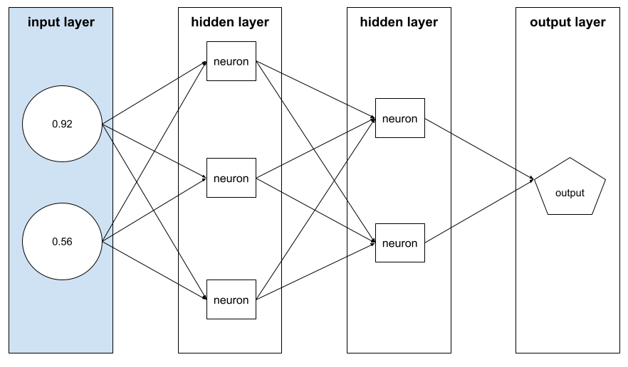
Each example supplies different values for the feature vector, so the feature vector for the next example could be something like:
[0.73, 0.49]
Feature engineering determines how to represent features in the feature vector. For example, a binary categorical feature with five possible values might be represented with one-hot encoding . In this case, the portion of the feature vector for a particular example would consist of four zeroes and a single 1.0 in the third position, as follows:
[0.0, 0.0, 1.0, 0.0, 0.0]
As another example, suppose your model consists of three features:
- a binary categorical feature with five possible values represented with one-hot encoding; for example:
[0.0, 1.0, 0.0, 0.0, 0.0] - another binary categorical feature with three possible values represented with one-hot encoding; for example:
[0.0, 0.0, 1.0] - a floating-point feature; for example:
8.3.
In this case, the feature vector for each example would be represented by nine values. Given the example values in the preceding list, the feature vector would be:
0.0
1.0
0.0
0.0
0.0
0.0
0.0
1.0
8.3
See Numerical data: How a model ingests data using feature vectors in Machine Learning Crash Course for more information.
featurization
The process of extracting features from an input source, such as a document or video, and mapping those features into a feature vector .
Some ML experts use featurization as a synonym for feature engineering or feature extraction .
federated learning
A distributed machine learning approach that trains machine learning models using decentralized examples residing on devices such as smartphones. In federated learning, a subset of devices downloads the current model from a central coordinating server. The devices use the examples stored on the devices to make improvements to the model. The devices then upload the model improvements (but not the training examples) to the coordinating server, where they are aggregated with other updates to yield an improved global model. After the aggregation, the model updates computed by devices are no longer needed, and can be discarded.
Since the training examples are never uploaded, federated learning follows the privacy principles of focused data collection and data minimization.
See the Federated Learning comic (yes, a comic) for more details.
обратная связь
A stage in an agentic loop in which the agent evaluates the action taken during the act stage. For example, if the agent sent an API request during the act stage, the feedback stage might determine whether the API response was successful.
feedback loop
In machine learning, a situation in which a model's predictions influence the training data for the same model or another model. For example, a model that recommends movies will influence the movies that people see, which will then influence subsequent movie recommendation models.
See Production ML systems: Questions to ask in Machine Learning Crash Course for more information.
feedforward neural network (FFN)
A neural network without cyclic or recursive connections. For example, traditional deep neural networks are feedforward neural networks. Contrast with recurrent neural networks , which are cyclic.
few-shot learning
A machine learning approach, often used for object classification, designed to train effective classification models from only a small number of training examples.
See also one-shot learning and zero-shot learning .
few-shot prompting
A prompt that contains more than one (a "few") example demonstrating how the large language model should respond. For example, the following lengthy prompt contains two examples showing a large language model how to answer a query.
| Parts of one prompt | Примечания |
|---|---|
| What is the official currency of the specified country? | The question you want the LLM to answer. |
| France: EUR | One example. |
| United Kingdom: GBP | Ещё один пример. |
| Индия: | The actual query. |
Few-shot prompting generally produces more desirable results than zero-shot prompting and one-shot prompting . However, few-shot prompting requires a lengthier prompt.
Few-shot prompting is a form of few-shot learning applied to prompt-based learning .
See Prompt engineering in Machine Learning Crash Course for more information.
Скрипка
A Python-first configuration library that sets the values of functions and classes without invasive code or infrastructure. In the case of Pax —and other ML codebases—these functions and classes represent models and training hyperparameters .
Fiddle assumes that machine learning codebases are typically divided into:
- Library code, which defines the layers and optimizers.
- Dataset "glue" code, which calls the libraries and wires everything together.
Fiddle captures the call structure of the glue code in an unevaluated and mutable form.
тонкая настройка
A second, task-specific training pass performed on a pre-trained model to refine its parameters for a specific use case. For example, the full training sequence for some large language models is as follows:
- Pre-training: Train a large language model on a vast general dataset, such as all the English language Wikipedia pages.
- Fine-tuning: Train the pre-trained model to perform a specific task, such as responding to medical queries. Fine-tuning typically involves hundreds or thousands of examples focused on the specific task.
As another example, the full training sequence for a large image model is as follows:
- Pre-training: Train a large image model on a vast general image dataset, such as all the images in Wikimedia commons.
- Fine-tuning: Train the pre-trained model to perform a specific task, such as generating images of orcas.
Fine-tuning can entail any combination of the following strategies:
- Modifying all of the pre-trained model's existing parameters . This is sometimes called full fine-tuning .
- Modifying only some of the pre-trained model's existing parameters (typically, the layers closest to the output layer ), while keeping other existing parameters unchanged (typically, the layers closest to the input layer ). See parameter-efficient tuning .
- Adding more layers, typically on top of the existing layers closest to the output layer.
Fine-tuning is a form of transfer learning . As such, fine-tuning might use a different loss function or a different model type than those used to train the pre-trained model. For example, you could fine-tune a pre-trained large image model to produce a regression model that returns the number of birds in an input image.
Compare and contrast fine-tuning with the following terms:
See Fine-tuning in Machine Learning Crash Course for more information.
Flash model
A family of relatively small Gemini models optimized for speed and low latency . Flash models are designed for a wide range of applications where quick responses and high throughput are crucial.
Лен
A high-performance open-source library for deep learning built on top of JAX . Flax provides functions for training neural networks , as well as methods for evaluating their performance.
Flaxformer
An open-source Transformer library , built on Flax , designed primarily for natural language processing and multimodal research.
forget gate
The portion of a Long Short-Term Memory cell that regulates the flow of information through the cell. Forget gates maintain context by deciding which information to discard from the cell state.
foundation model
A very large pre-trained model trained on an enormous and diverse training set . A foundation model can do both of the following:
- Respond well to a wide range of requests.
- Serve as a base model for additional fine-tuning or other customization.
In other words, a foundation model is already very capable in a general sense but can be further customized to become even more useful for a specific task.
fraction of successes
A metric for evaluating an ML model's generated text . The fraction of successes is the number of "successful" generated text outputs divided by the total number of generated text outputs. For example, if a large language model generated 10 blocks of code, five of which were successful, then the fraction of successes would be 50%.
Although fraction of successes is broadly useful throughout statistics, within ML, this metric is primarily useful for measuring verifiable tasks like code generation or math problems.
full softmax
Synonym for softmax .
Contrast with candidate sampling .
See Neural networks: Multi-class classification in Machine Learning Crash Course for more information.
fully connected layer
A hidden layer in which each node is connected to every node in the subsequent hidden layer.
A fully connected layer is also known as a dense layer .
function transformation
A function that takes a function as input and returns a transformed function as output. JAX uses function transformations.
Г
ГАН
Abbreviation for generative adversarial network .
Близнецы
The ecosystem comprising Google's most advanced AI. Elements of this ecosystem include:
- Various Gemini models .
- The interactive conversational interface to a Gemini model. Users type prompts and Gemini responds to those prompts.
- Various Gemini APIs.
- Various business products based on Gemini models; for example, Gemini for Google Cloud .
модели Близнецов
Google's state-of-the-art Transformer -based multimodal models . Gemini models are specifically designed to integrate with agents .
Users can interact with Gemini models in a variety of ways, including through an interactive dialog interface and through SDKs.
Джемма
A family of lightweight open models built from the same research and technology used to create the Gemini models. Several different Gemma models are available, each providing different features, such as vision, code, and instruction following. See Gemma for details.
GenAI or genAI
Abbreviation for generative AI .
обобщение
A model's ability to make correct predictions on new, previously unseen data. A model that can generalize is the opposite of a model that is overfitting .
See Generalization in Machine Learning Crash Course for more information.
generalization curve
A plot of both training loss and validation loss as a function of the number of iterations .
A generalization curve can help you detect possible overfitting . For example, the following generalization curve suggests overfitting because validation loss ultimately becomes significantly higher than training loss.
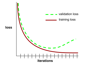
See Generalization in Machine Learning Crash Course for more information.
generalized linear model
A generalization of least squares regression models, which are based on Gaussian noise , to other types of models based on other types of noise, such as Poisson noise or categorical noise. Examples of generalized linear models include:
- logistic regression
- multi-class regression
- least squares regression
The parameters of a generalized linear model can be found through convex optimization .
Generalized linear models exhibit the following properties:
- The average prediction of the optimal least squares regression model is equal to the average label on the training data.
- The average probability predicted by the optimal logistic regression model is equal to the average label on the training data.
The power of a generalized linear model is limited by its features. Unlike a deep model, a generalized linear model cannot "learn new features."
generated text
In general, the text that an ML model outputs. When evaluating large language models, some metrics compare generated text against reference text . For example, suppose you are trying to determine how effectively an ML model translates from French to Dutch. In this case:
- The generated text is the Dutch translation that the ML model outputs.
- The reference text is the Dutch translation that a human translator (or software) creates.
Note that some evaluation strategies don't involve reference text.
generative adversarial network (GAN)
A system to create new data in which a generator creates data and a discriminator determines whether that created data is valid or invalid.
See the Generative Adversarial Networks course for more information.
generative agents (simulacra)
Agents endowed with unique personas, memories, and routines that simulate realistic human behavior.
See Generative Agents: Interactive Simulacra of Human Behavior for details.
generative AI
An emerging transformative field with no formal definition. That said, most experts agree that generative AI models can create ("generate") content that is all of the following:
- сложный
- согласованный
- оригинал
Examples of generative AI include:
- Large language models , which can generate sophisticated original text and answer questions.
- Image generation model, which can produce unique images.
- Audio and music generation models, which can compose original music or generate realistic speech.
- Video generation models, which can generate original videos.
Some earlier technologies, including LSTMs and RNNs , can also generate original and coherent content. Some experts view these earlier technologies as generative AI, while others feel that true generative AI requires more complex output than those earlier technologies can produce.
Contrast with predictive ML .
generative model
Practically speaking, a model that does either of the following:
- Creates (generates) new examples from the training dataset. For example, a generative model could create poetry after training on a dataset of poems. The generator part of a generative adversarial network falls into this category.
- Determines the probability that a new example comes from the training set, or was created from the same mechanism that created the training set. For example, after training on a dataset consisting of English sentences, a generative model could determine the probability that new input is a valid English sentence.
A generative model can theoretically discern the distribution of examples or particular features in a dataset. That is:
p(examples)
Unsupervised learning models are generative.
Contrast with discriminative models .
генератор
The subsystem within a generative adversarial network that creates new examples .
Contrast with discriminative model .
gini impurity
A metric similar to entropy . Splitters use values derived from either gini impurity or entropy to compose conditions for classification decision trees . Information gain is derived from entropy. No universally accepted equivalent term for the metric derived from gini impurity exists; however, this unnamed metric is just as important as information gain.
Gini impurity is also called gini index , or simply gini .
golden dataset
A set of manually curated data that captures ground truth . Teams can use one or more golden datasets to evaluate a model's quality.
Some golden datasets capture different subdomains of ground truth. For example, a golden dataset for image classification might capture lighting conditions and image resolution.
golden response
A response known to be good. For example, given the following prompt :
2 + 2
The golden response is hopefully:
4
Google AI Studio
A Google tool providing a user-friendly interface for experimenting with and building applications using Google's large language models . See the Google AI Studio home page for details.
GPT (Generative Pre-trained Transformer)
A family of Transformer -based large language models developed by OpenAI .
GPT variants can apply to multiple modalities , including:
- image generation (for example, ImageGPT)
- text-to-image generation (for example, DALL-E ).
градиент
The vector of partial derivatives with respect to all of the independent variables. In machine learning, the gradient is the vector of partial derivatives of the model function. The gradient points in the direction of steepest ascent.
gradient accumulation
A backpropagation technique that updates the parameters only once per epoch rather than once per iteration. After processing each mini-batch , gradient accumulation simply updates a running total of gradients. Then, after processing the last mini-batch in the epoch, the system finally updates the parameters based on the total of all gradient changes.
Gradient accumulation is useful when the batch size is very large compared to the amount of available memory for training. When memory is an issue, the natural tendency is to reduce batch size. However, reducing the batch size in normal backpropagation increases the number of parameter updates. Gradient accumulation enables the model to avoid memory issues but still train efficiently.
gradient boosted (decision) trees (GBT)
A type of decision forest in which:
- Training relies on gradient boosting .
- The weak model is a decision tree .
See Gradient Boosted Decision Trees in the Decision Forests course for more information.
gradient boosting
A training algorithm where weak models are trained to iteratively improve the quality (reduce the loss) of a strong model. For example, a weak model could be a linear or small decision tree model. The strong model becomes the sum of all the previously trained weak models.
In the simplest form of gradient boosting, at each iteration, a weak model is trained to predict the loss gradient of the strong model. Then, the strong model's output is updated by subtracting the predicted gradient, similar to gradient descent .
где:
- $F_{0}$ is the starting strong model.
- $F_{i+1}$ is the next strong model.
- $F_{i}$ is the current strong model.
- $\xi$ is a value between 0.0 and 1.0 called shrinkage , which is analogous to the learning rate in gradient descent.
- $f_{i}$ is the weak model trained to predict the loss gradient of $F_{i}$.
Modern variations of gradient boosting also include the second derivative (Hessian) of the loss in their computation.
Decision trees are commonly used as weak models in gradient boosting. See gradient boosted (decision) trees .
gradient clipping
A commonly used mechanism to mitigate the exploding gradient problem by artificially limiting (clipping) the maximum value of gradients when using gradient descent to train a model.
градиентный спуск
A mathematical technique to minimize loss . Gradient descent iteratively adjusts weights and biases , gradually finding the best combination to minimize loss.
Gradient descent is older—much, much older—than machine learning.
See the Linear regression: Gradient descent in Machine Learning Crash Course for more information.
график
In TensorFlow, a computation specification. Nodes in the graph represent operations. Edges are directed and represent passing the result of an operation (a Tensor ) as an operand to another operation. Use TensorBoard to visualize a graph.
graph execution
A TensorFlow programming environment in which the program first constructs a graph and then executes all or part of that graph. Graph execution is the default execution mode in TensorFlow 1.x.
Contrast with eager execution .
greedy policy
In reinforcement learning, a policy that always chooses the action with the highest expected return .
обоснованность
A property of a model whose output is based on (is "grounded on") specific source material. For example, suppose you provide an entire physics textbook as input ("context") to a large language model . Then, you prompt that large language model with a physics question. If the model's response reflects information in that textbook, then that model is grounded on that textbook.
Note that a grounded model is not always a factual model. For example, the input physics textbook could contain mistakes.
заземление
The process of basing all or part of an LLM's response on information retrieved from one or more trusted sources. For example, suppose a user prompts an LLM for today's weather forecast in Berlin. The LLM might ground the response on information it gathers from the European Centre for Medium-Range Weather Forecasts.
Retrieval-augmented generation (RAG) is a common grounding technique.
ground truth
Реальность.
The thing that actually happened.
For example, consider a binary classification model that predicts whether a student in their first year of university will graduate within six years. Ground truth for this model is whether or not that student actually graduated within six years.
group attribution bias
Assuming that what is true for an individual is also true for everyone in that group. The effects of group attribution bias can be exacerbated if a convenience sampling is used for data collection. In a non-representative sample, attributions may be made that don't reflect reality.
See also out-group homogeneity bias and in-group bias . Also, see Fairness: Types of bias in Machine Learning Crash Course for more information.
ограждения
Any software or process that prevents harm to humans or systems. Harm can take many forms, including preventing data leaks or unauthorized access, or ensuring that an LLM's responses don't contain offensive material.
ЧАС
галлюцинация
The production of plausible-seeming but factually incorrect output by a generative AI model that purports to be making an assertion about the real world. For example, a generative AI model that claims that Barack Obama died in 1865 is hallucinating .
хеширование
In machine learning, a mechanism for bucketing categorical data , particularly when the number of categories is large, but the number of categories actually appearing in the dataset is comparatively small.
For example, Earth is home to about 73,000 tree species. You could represent each of the 73,000 tree species in 73,000 separate categorical buckets. Alternatively, if only 200 of those tree species actually appear in a dataset, you could use hashing to divide tree species into perhaps 500 buckets.
A single bucket could contain multiple tree species. For example, hashing could place baobab and red maple —two genetically dissimilar species—into the same bucket. Regardless, hashing is still a good way to map large categorical sets into the selected number of buckets. Hashing turns a categorical feature having a large number of possible values into a much smaller number of values by grouping values in a deterministic way.
See Categorical data: Vocabulary and one-hot encoding in Machine Learning Crash Course for more information.
эвристический
A simple and quickly implemented solution to a problem. For example, "With a heuristic, we achieved 86% accuracy. When we switched to a deep neural network, accuracy went up to 98%."
скрытый слой
A layer in a neural network between the input layer (the features) and the output layer (the prediction). Each hidden layer consists of one or more neurons . For example, the following neural network contains two hidden layers, the first with three neurons and the second with two neurons:
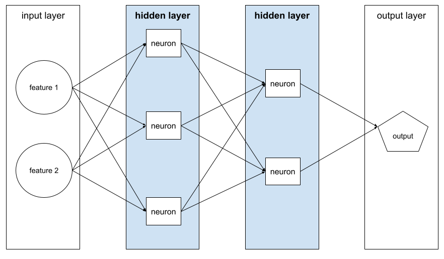
A deep neural network contains more than one hidden layer. For example, the preceding illustration is a deep neural network because the model contains two hidden layers.
See Neural networks: Nodes and hidden layers in Machine Learning Crash Course for more information.
иерархическая кластеризация
A category of clustering algorithms that create a tree of clusters. Hierarchical clustering is well-suited to hierarchical data, such as botanical taxonomies. There are two types of hierarchical clustering algorithms:
- Agglomerative clustering first assigns every example to its own cluster, and iteratively merges the closest clusters to create a hierarchical tree.
- Divisive clustering first groups all examples into one cluster and then iteratively divides the cluster into a hierarchical tree.
Contrast with centroid-based clustering .
See Clustering algorithms in the Clustering course for more information.
hill climbing
An algorithm for iteratively improving ("walking uphill") an ML model until the model stops improving ("reaches the top of a hill"). The general form of the algorithm is as follows:
- Build a starting model.
- Create new candidate models by making small adjustments to the way you train or fine-tune . This might entail working with a slightly different training set or different hyperparameters.
- Evaluate the new candidate models and take one of the following actions:
- If a candidate model outperforms the starting model, then that candidate model becomes the new starting model. In this case, repeat Steps 1, 2, and 3.
- If no model outperforms the starting model, then you've reached the top of the hill and should stop iterating.
See Deep Learning Tuning Playbook for guidance on hyperparameter tuning. See the Data modules of Machine Learning Crash Course for guidance on feature engineering.
потеря шарнира
A family of loss functions for classification designed to find the decision boundary as distant as possible from each training example, thus maximizing the margin between examples and the boundary. KSVMs use hinge loss (or a related function, such as squared hinge loss). For binary classification, the hinge loss function is defined as follows:
where y is the true label, either -1 or +1, and y' is the raw output of the classification model :
Consequently, a plot of hinge loss versus (y * y') looks as follows:

historical bias
A type of bias that already exists in the world and has made its way into a dataset. These biases have a tendency to reflect existing cultural stereotypes, demographic inequalities, and prejudices against certain social groups.
For example, consider a classification model that predicts whether or not a loan applicant will default on their loan, which was trained on historical loan-default data from the 1980s from local banks in two different communities. If past applicants from Community A were six times more likely to default on their loans than applicants from Community B, the model might learn a historical bias resulting in the model being less likely to approve loans in Community A, even if the historical conditions that resulted in that community's higher default rates were no longer relevant.
See Fairness: Types of bias in Machine Learning Crash Course for more information.
holdout data
Examples intentionally not used ("held out") during training. The validation dataset and test dataset are examples of holdout data. Holdout data helps evaluate your model's ability to generalize to data other than the data it was trained on. The loss on the holdout set provides a better estimate of the loss on an unseen dataset than does the loss on the training set.
хозяин
When training an ML model on accelerator chips (GPUs or TPUs ), the part of the system that controls both of the following:
- The overall flow of the code.
- The extraction and transformation of the input pipeline.
The host typically runs on a CPU, not on an accelerator chip; the device manipulates tensors on the accelerator chips.
human evaluation
A process in which people judge the quality of an ML model's output; for example, having bilingual people judge the quality of an ML translation model. Human evaluation is particularly useful for judging models that have no one right answer .
Contrast with automatic evaluation and autorater evaluation .
human in the loop (HITL)
A loosely-defined idiom that could mean either of the following:
- A policy of viewing generative AI output critically or skeptically.
- A strategy or system for ensuring that people help shape, evaluate, and refine a model's behavior. Keeping a human in the loop enables an AI to benefit from both machine intelligence and human intelligence. For example, a system in which an AI generates code which software engineers then review is a human-in-the-loop system.
hyperparameter
The variables that you or a hyperparameter tuning serviceadjust during successive runs of training a model. For example, learning rate is a hyperparameter. You could set the learning rate to 0.01 before one training session. If you determine that 0.01 is too high, you could perhaps set the learning rate to 0.003 for the next training session.
In contrast, parameters are the various weights and bias that the model learns during training.
See Linear regression: Hyperparameters in Machine Learning Crash Course for more information.
hyperplane
A boundary that separates a space into two subspaces. For example, a line is a hyperplane in two dimensions and a plane is a hyperplane in three dimensions. More typically in machine learning, a hyperplane is the boundary separating a high-dimensional space. Kernel Support Vector Machines use hyperplanes to separate positive classes from negative classes, often in a very high-dimensional space.
я
иид
Abbreviation for independently and identically distributed .
распознавание изображений
A process that classifies object(s), pattern(s), or concept(s) in an image. Image recognition is also known as image classification .
imbalanced dataset
Synonym for class-imbalanced dataset .
неявная предвзятость
Automatically making an association or assumption based on one's mind models and memories. Implicit bias can affect the following:
- How data is collected and classified.
- How machine learning systems are designed and developed.
For example, when building a classification model to identify wedding photos, an engineer may use the presence of a white dress in a photo as a feature. However, white dresses have been customary only during certain eras and in certain cultures.
See also confirmation bias .
imputation
Short form of value imputation .
incompatibility of fairness metrics
The idea that some notions of fairness are mutually incompatible and cannot be satisfied simultaneously. As a result, there is no single universal metric for quantifying fairness that can be applied to all ML problems.
While this may seem discouraging, incompatibility of fairness metrics doesn't imply that fairness efforts are fruitless. Instead, it suggests that fairness must be defined contextually for a given ML problem, with the goal of preventing harms specific to its use cases.
See "On the (im)possibility of fairness" for a more detailed discussion of the incompatibility of fairness metrics.
in-context learning
Synonym for few-shot prompting .
independently and identically distributed (iid)
Data drawn from a distribution that doesn't change, and where each value drawn doesn't depend on values that have been drawn previously. An iid is the ideal gas of machine learning—a useful mathematical construct but almost never exactly found in the real world. For example, the distribution of visitors to a web page may be iid over a brief window of time; that is, the distribution doesn't change during that brief window and one person's visit is generally independent of another's visit. However, if you expand that window of time, seasonal differences in the web page's visitors may appear.
See also nonstationarity .
individual fairness
A fairness metric that checks whether similar individuals are classified similarly. For example, Brobdingnagian Academy might want to satisfy individual fairness by ensuring that two students with identical grades and standardized test scores are equally likely to gain admission.
Note that individual fairness relies entirely on how you define "similarity" (in this case, grades and test scores), and you can run the risk of introducing new fairness problems if your similarity metric misses important information (such as the rigor of a student's curriculum).
See "Fairness Through Awareness" for a more detailed discussion of individual fairness.
вывод
In traditional machine learning, the process of making predictions by applying a trained model to unlabeled examples . See Supervised Learning in the Intro to ML course to learn more.
In large language models , inference is the process of using a trained model to generate a response to an input prompt .
Inference has a somewhat different meaning in statistics. See the Wikipedia article on statistical inference for details.
inference path
In a decision tree , during inference , the route a particular example takes from the root to other conditions , terminating with a leaf . For example, in the following decision tree, the thicker arrows show the inference path for an example with the following feature values:
- x = 7
- y = 12
- z = -3
The inference path in the following illustration travels through three conditions before reaching the leaf ( Zeta ).
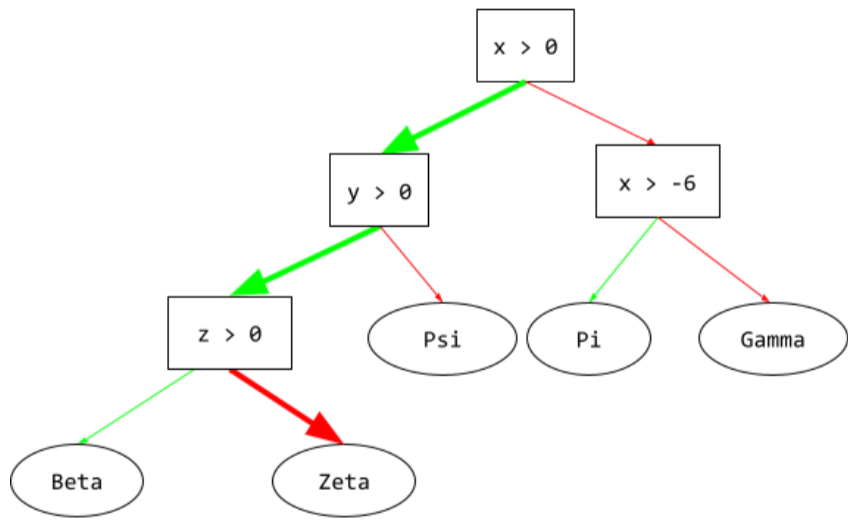
The three thick arrows show the inference path.
See Decision trees in the Decision Forests course for more information.
information gain
In decision forests , the difference between a node's entropy and the weighted (by number of examples) sum of the entropy of its children nodes. A node's entropy is the entropy of the examples in that node.
For example, consider the following entropy values:
- entropy of parent node = 0.6
- entropy of one child node with 16 relevant examples = 0.2
- entropy of another child node with 24 relevant examples = 0.1
So 40% of the examples are in one child node and 60% are in the other child node. Therefore:
- weighted entropy sum of child nodes = (0.4 * 0.2) + (0.6 * 0.1) = 0.14
So, the information gain is:
- information gain = entropy of parent node - weighted entropy sum of child nodes
- information gain = 0.6 - 0.14 = 0.46
Most splitters seek to create conditions that maximize information gain.
in-group bias
Showing partiality to one's own group or own characteristics. If testers or raters consist of the machine learning developer's friends, family, or colleagues, then in-group bias may invalidate product testing or the dataset.
In-group bias is a form of group attribution bias . See also out-group homogeneity bias .
See Fairness: Types of bias in Machine Learning Crash Course for more information.
input generator
A mechanism by which data is loaded into a neural network .
An input generator can be thought of as a component responsible for processing raw data into tensors which are iterated over to generate batches for training, evaluation, and inference.
input layer
The layer of a neural network that holds the feature vector . That is, the input layer provides examples for training or inference . For example, the input layer in the following neural network consists of two features:

in-set condition
In a decision tree , a condition that tests for the presence of one item in a set of items. For example, the following is an in-set condition:
house-style in [tudor, colonial, cape]
During inference, if the value of the house-style feature is tudor or colonial or cape , then this condition evaluates to Yes. If the value of the house-style feature is something else (for example, ranch ), then this condition evaluates to No.
In-set conditions usually lead to more efficient decision trees than conditions that test one-hot encoded features.
пример
Synonym for example .
instruction tuning
A form of fine-tuning that improves a generative AI model's ability to follow instructions. Instruction tuning involves training a model on a series of instruction prompts, typically covering a wide variety of tasks. The resulting instruction-tuned model then tends to generate useful responses to zero-shot prompts across a variety of tasks.
Compare and contrast with:
интерпретируемость
The ability to explain or to present an ML model's reasoning in understandable terms to a human.
Most linear regression models, for example, are highly interpretable. (You merely need to look at the trained weights for each feature.) Decision forests are also highly interpretable. Some models, however, require sophisticated visualization to become interpretable.
You can use the Learning Interpretability Tool (LIT) to interpret ML models.
inter-rater agreement
A measurement of how often human raters agree when doing a task. If raters disagree, the task instructions may need to be improved. Also sometimes called inter-annotator agreement or inter-rater reliability . See also Cohen's kappa , which is one of the most popular inter-rater agreement measurements.
See Categorical data: Common issues in Machine Learning Crash Course for more information.
intersection over union (IoU)
The intersection of two sets divided by their union. In machine-learning image-detection tasks, IoU is used to measure the accuracy of the model's predicted bounding box with respect to the ground-truth bounding box. In this case, the IoU for the two boxes is the ratio between the overlapping area and the total area, and its value ranges from 0 (no overlap of predicted bounding box and ground-truth bounding box) to 1 (predicted bounding box and ground-truth bounding box have the exact same coordinates).
For example, in the image below:
- The predicted bounding box (the coordinates delimiting where the model predicts the night table in the painting is located) is outlined in purple.
- The ground-truth bounding box (the coordinates delimiting where the night table in the painting is actually located) is outlined in green.
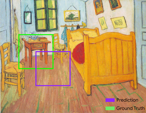
Here, the intersection of the bounding boxes for prediction and ground truth (below left) is 1, and the union of the bounding boxes for prediction and ground truth (below right) is 7, so the IoU is \(\frac{1}{7}\).
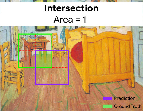
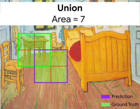
IoU
Abbreviation for intersection over union .
item matrix
In recommendation systems , a matrix of embedding vectors generated by matrix factorization that holds latent signals about each item . Each row of the item matrix holds the value of a single latent feature for all items. For example, consider a movie recommendation system. Each column in the item matrix represents a single movie. The latent signals might represent genres, or might be harder-to-interpret signals that involve complex interactions among genre, stars, movie age, or other factors.
The item matrix has the same number of columns as the target matrix that is being factorized. For example, given a movie recommendation system that evaluates 10,000 movie titles, the item matrix will have 10,000 columns.
предметы
In a recommendation system , the entities that a system recommends. For example, videos are the items that a video store recommends, while books are the items that a bookstore recommends.
итерация
A single update of a model's parameters—the model's weights and biases —during training . The batch size determines how many examples the model processes in a single iteration. For instance, if the batch size is 20, then the model processes 20 examples before adjusting the parameters.
When training a neural network , a single iteration involves the following two passes:
- A forward pass to evaluate loss on a single batch.
- A backward pass ( backpropagation ) to adjust the model's parameters based on the loss and the learning rate.
See Gradient descent in Machine Learning Crash Course for more information.
Дж.
ДЖАКС
An array computing library, bringing together XLA (Accelerated Linear Algebra) and automatic differentiation for high-performance numerical computing. JAX provides a simple and powerful API for writing accelerated numerical code with composable transformations. JAX provides features such as:
-
grad(automatic differentiation) -
jit(just-in-time compilation) -
vmap(automatic vectorization or batching) -
pmap(parallelization)
JAX is a language for expressing and composing transformations of numerical code, analogous—but much larger in scope—to Python's NumPy library. (In fact, the .numpy library under JAX is a functionally equivalent, but entirely rewritten version of the Python NumPy library.)
JAX is particularly well-suited for speeding up many machine learning tasks by transforming the models and data into a form suitable for parallelism across GPU and TPU accelerator chips .
Flax , Optax , Pax , and many other libraries are built on the JAX infrastructure.
К
Керас
A popular Python machine learning API. Keras runs on several deep learning frameworks, including TensorFlow, where it is made available as tf.keras .
Kernel Support Vector Machines (KSVMs)
A classification algorithm that seeks to maximize the margin between positive and negative classes by mapping input data vectors to a higher dimensional space. For example, consider a classification problem in which the input dataset has a hundred features. To maximize the margin between positive and negative classes, a KSVM could internally map those features into a million-dimension space. KSVMs uses a loss function called hinge loss .
keypoints
The coordinates of particular features in an image. For example, for an image recognition model that distinguishes flower species, keypoints might be the center of each petal, the stem, the stamen, and so on.
k-fold cross validation
An algorithm for predicting a model's ability to generalize to new data. The k in k-fold refers to the number of equal groups you divide a dataset's examples into; that is, you train and test your model k times. For each round of training and testing, a different group is the test set, and all remaining groups become the training set. After k rounds of training and testing, you calculate the mean and standard deviation of the chosen test metric(s).
For example, suppose your dataset consists of 120 examples. Further suppose, you decide to set k to 4. Therefore, after shuffling the examples, you divide the dataset into four equal groups of 30 examples and conduct four training and testing rounds:
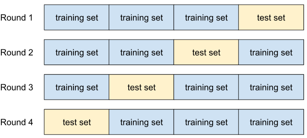
For example, Mean Squared Error (MSE) might be the most meaningful metric for a linear regression model. Therefore, you would find the mean and standard deviation of the MSE across all four rounds.
k-means
A popular clustering algorithm that groups examples in unsupervised learning. The k-means algorithm basically does the following:
- Iteratively determines the best k center points (known as centroids ).
- Assigns each example to the closest centroid. Those examples nearest the same centroid belong to the same group.
The k-means algorithm picks centroid locations to minimize the cumulative square of the distances from each example to its closest centroid.
For example, consider the following plot of dog height to dog width:

If k=3, the k-means algorithm will determine three centroids. Each example is assigned to its closest centroid, yielding three groups:

Imagine that a manufacturer wants to determine the ideal sizes for small, medium, and large sweaters for dogs. The three centroids identify the mean height and mean width of each dog in that cluster. So, the manufacturer should probably base sweater sizes on those three centroids. Note that the centroid of a cluster is typically not an example in the cluster.
The preceding illustrations shows k-means for examples with only two features (height and width). Note that k-means can group examples across many features.
See What is k-means clustering? in the Clustering course for more information.
k-median
A clustering algorithm closely related to k-means . The practical difference between the two is as follows:
- In k-means, centroids are determined by minimizing the sum of the squares of the distance between a centroid candidate and each of its examples.
- In k-median, centroids are determined by minimizing the sum of the distance between a centroid candidate and each of its examples.
Note that the definitions of distance are also different:
- k-means relies on the Euclidean distance from the centroid to an example. (In two dimensions, the Euclidean distance means using the Pythagorean theorem to calculate the hypotenuse.) For example, the k-means distance between (2,2) and (5,-2) would be:
- k-median relies on the Manhattan distance from the centroid to an example. This distance is the sum of the absolute deltas in each dimension. For example, the k-median distance between (2,2) and (5,-2) would be:
Л
L 0 regularization
A type of regularization that penalizes the total number of nonzero weights in a model. For example, a model having 11 nonzero weights would be penalized more than a similar model having 10 nonzero weights.
L 0 regularization is sometimes called L0-norm regularization .
L 1 loss
A loss function that calculates the absolute value of the difference between actual label values and the values that a model predicts. For example, here's the calculation of L 1 loss for a batch of five examples :
| Actual value of example | Model's predicted value | Absolute value of delta |
|---|---|---|
| 7 | 6 | 1 |
| 5 | 4 | 1 |
| 8 | 11 | 3 |
| 4 | 6 | 2 |
| 9 | 8 | 1 |
| 8 = L 1 loss | ||
L 1 loss is less sensitive to outliers than L 2 loss .
The Mean Absolute Error is the average L 1 loss per example.
See Linear regression: Loss in Machine Learning Crash Course for more information.
L1- регуляризация
A type of regularization that penalizes weights in proportion to the sum of the absolute value of the weights. L 1 regularization helps drive the weights of irrelevant or barely relevant features to exactly 0 . A feature with a weight of 0 is effectively removed from the model.
Contrast with L 2 regularization .
L 2 loss
A loss function that calculates the square of the difference between actual label values and the values that a model predicts. For example, here's the calculation of L 2 loss for a batch of five examples :
| Actual value of example | Model's predicted value | Square of delta |
|---|---|---|
| 7 | 6 | 1 |
| 5 | 4 | 1 |
| 8 | 11 | 9 |
| 4 | 6 | 4 |
| 9 | 8 | 1 |
| 16 = L 2 loss | ||
Due to squaring, L 2 loss amplifies the influence of outliers . That is, L 2 loss reacts more strongly to bad predictions than L 1 loss . For example, the L 1 loss for the preceding batch would be 8 rather than 16. Notice that a single outlier accounts for 9 of the 16.
Regression models typically use L 2 loss as the loss function.
The Mean Squared Error is the average L 2 loss per example. Squared loss is another name for L 2 loss.
See Logistic regression: Loss and regularization in Machine Learning Crash Course for more information.
L2- регуляризация
A type of regularization that penalizes weights in proportion to the sum of the squares of the weights. L 2 regularization helps drive outlier weights (those with high positive or low negative values) closer to 0 but not quite to 0 . Features with values very close to 0 remain in the model but don't influence the model's prediction very much.
L 2 regularization always improves generalization in linear models .
Contrast with L 1 regularization .
See Overfitting: L2 regularization in Machine Learning Crash Course for more information.
этикетка
In supervised machine learning , the "answer" or "result" portion of an example .
Each labeled example consists of one or more features and a label. For example, in a spam detection dataset, the label would probably be either "spam" or "not spam." In a rainfall dataset, the label might be the amount of rain that fell during a certain period.
See Supervised Learning in Introduction to Machine Learning for more information.
labeled example
An example that contains one or more features and a label . For example, the following table shows three labeled examples from a house valuation model, each with three features and one label:
| Количество спален | Количество ванных комнат | House age | House price (label) |
|---|---|---|---|
| 3 | 2 | 15 | $345,000 |
| 2 | 1 | 72 | 179 000 долларов США |
| 4 | 2 | 34 | $392,000 |
In supervised machine learning , models train on labeled examples and make predictions on unlabeled examples .
Contrast labeled example with unlabeled examples.
See Supervised Learning in Introduction to Machine Learning for more information.
label leakage
A model design flaw in which a feature is a proxy for the label . For example, consider a binary classification model that predicts whether or not a prospective customer will purchase a particular product. Suppose that one of the features for the model is a Boolean named SpokeToCustomerAgent . Further suppose that a customer agent is only assigned after the prospective customer has actually purchased the product. During training, the model will quickly learn the association between SpokeToCustomerAgent and the label.
See Monitoring pipelines in Machine Learning Crash Course for more information.
лямбда
Synonym for regularization rate .
Lambda is an overloaded term. Here we're focusing on the term's definition within regularization .
LaMDA (Language Model for Dialogue Applications)
A Transformer -based large language model developed by Google trained on a large dialogue dataset that can generate realistic conversational responses .
LaMDA: our breakthrough conversation technology provides an overview.
достопримечательности
Synonym for keypoints .
language model
A model that estimates the probability of a token or sequence of tokens occurring in a longer sequence of tokens.
See What is a language model? in Machine Learning Crash Course for more information.
большая языковая модель
At a minimum, a language model having a very high number of parameters . More informally, any Transformer -based language model, such as Gemini or GPT .
See Large language models (LLMs) in Machine Learning Crash Course for more information.
задержка
The time it takes for a model to process input and generate a response. A high latency response takes takes longer to generate than a low latency response.
Factors that influence latency of large language models include:
- Input and output token lengths
- Model complexity
- The infrastructure the model runs on
Optimizing for latency is crucial for creating responsive and user-friendly applications.
скрытое пространство
Synonym for embedding space .
слой
A set of neurons in a neural network . Three common types of layers are as follows:
- The input layer , which provides values for all the features .
- One or more hidden layers , which find nonlinear relationships between the features and the label.
- The output layer , which provides the prediction.
For example, the following illustration shows a neural network with one input layer, two hidden layers, and one output layer:
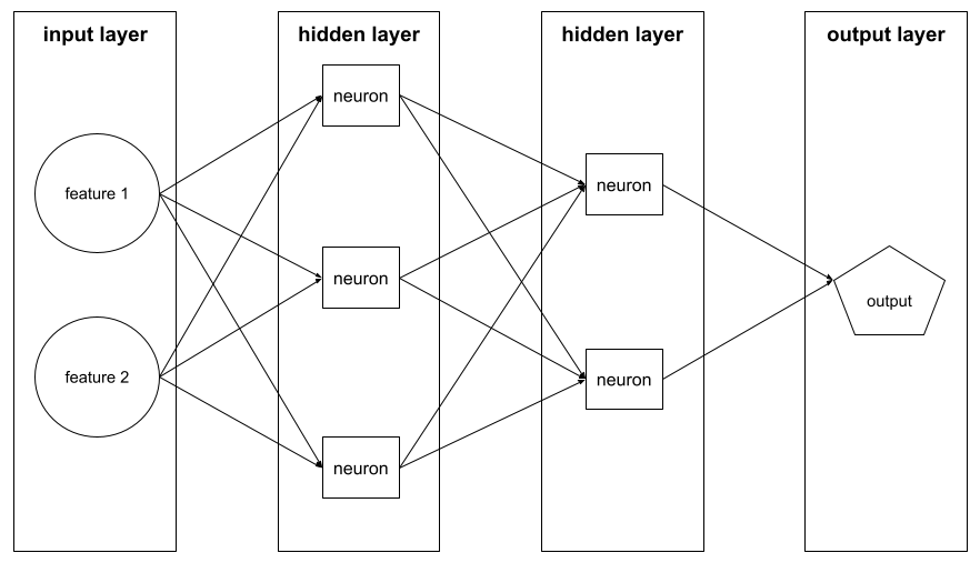
In TensorFlow , layers are also Python functions that take Tensors and configuration options as input and produce other tensors as output.
Layers API (tf.layers)
A TensorFlow API for constructing a deep neural network as a composition of layers. The Layers API lets you build different types of layers , such as:
-
tf.layers.Densefor a fully-connected layer . -
tf.layers.Conv2Dfor a convolutional layer.
The Layers API follows the Keras layers API conventions. That is, aside from a different prefix, all functions in the Layers API have the same names and signatures as their counterparts in the Keras layers API.
лист
Any endpoint in a decision tree . Unlike a condition , a leaf doesn't perform a test. Rather, a leaf is a possible prediction. A leaf is also the terminal node of an inference path .
For example, the following decision tree contains three leaves:
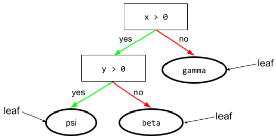
See Decision trees in the Decision Forests course for more information.
Learning Interpretability Tool (LIT)
A visual, interactive model-understanding and data visualization tool.
You can use open-source LIT to interpret models or to visualize text, image, and tabular data.
скорость обучения
A floating-point number that tells the gradient descent algorithm how strongly to adjust weights and biases on each iteration . For example, a learning rate of 0.3 would adjust weights and biases three times more powerfully than a learning rate of 0.1.
Learning rate is a key hyperparameter . If you set the learning rate too low, training will take too long. If you set the learning rate too high, gradient descent often has trouble reaching convergence .
See Linear regression: Hyperparameters in Machine Learning Crash Course for more information.
least squares regression
A linear regression model trained by minimizing L 2 Loss .
least-to-most prompting
A form of prompt chaining that divides complex problems into an ordered set of simpler problems. For example, here's a least-to-most prompting strategy for a certain problem:
- Divide a complex problem into an ordered list of simpler sub-problems. For this example, assume it is three sub-problems.
- Prompt 1: Ask the LLM to solve the first sub-problem. The LLM returns Response 1.
- Prompt 2: Integrate all or part of Response 1 into the prompt to solve the second sub-problem. The LLM returns Response 2.
- Prompt 3: Integrate all or part of Response 2 into the prompt to solve the third sub-problem. The LLM's response to Prompt 3 is the "final" answer to the initial complex problem.
Note that each step depends on the solution to the preceding step.
Contrast with tree-of-thought prompting .
Levenshtein Distance
An edit distance metric that calculates the fewest delete, insert, and substitute operations required to change one word to another. For example, the Levenshtein distance between the words "heart" and "darts" is three because the following three edits are the fewest changes to turn one word into the other:
- heart → deart (substitute "h" with "d")
- deart → dart (delete "e")
- dart → darts (insert "s")
Note that the preceding sequence isn't the only path of three edits.
линейный
A relationship between two or more variables that can be represented solely through addition and multiplication.
The plot of a linear relationship is a line.
Contrast with nonlinear .
linear model
A model that assigns one weight per feature to make predictions . (Linear models also incorporate a bias .) In contrast, the relationship of features to predictions in deep models is generally nonlinear .
Linear models are usually easier to train and more interpretable than deep models. However, deep models can learn complex relationships between features.
Linear regression and logistic regression are two types of linear models.
linear regression
A type of machine learning model in which both of the following are true:
- The model is a linear model .
- The prediction is a floating-point value. (This is the regression part of linear regression .)
Contrast linear regression with logistic regression . Also, contrast regression with classification .
See Linear regression in Machine Learning Crash Course for more information.
ЛИТ
Abbreviation for the Learning Interpretability Tool (LIT) , which was previously known as the Language Interpretability Tool.
магистр права
Abbreviation for large language model .
LLM evaluations (evals)
A set of metrics and benchmarks for assessing the performance of large language models (LLMs). At a high level, LLM evaluations:
- Help researchers identify areas where LLMs need improvement.
- Are useful in comparing different LLMs and identifying the best LLM for a particular task.
- Help ensure that LLMs are safe and ethical to use.
See Large language models (LLMs) in Machine Learning Crash Course for more information.
logistic regression
A type of regression model that predicts a probability. Logistic regression models have the following characteristics:
- The label is categorical . The term logistic regression usually refers to binary logistic regression , that is, to a model that calculates probabilities for labels with two possible values. A less common variant, multinomial logistic regression , calculates probabilities for labels with more than two possible values.
- The loss function during training is Log Loss . (Multiple Log Loss units can be placed in parallel for labels with more than two possible values.)
- The model has a linear architecture, not a deep neural network. However, the remainder of this definition also applies to deep models that predict probabilities for categorical labels.
For example, consider a logistic regression model that calculates the probability of an input email being either spam or not spam. During inference, suppose the model predicts 0.72. Therefore, the model is estimating:
- A 72% chance of the email being spam.
- A 28% chance of the email not being spam.
A logistic regression model uses the following two-step architecture:
- The model generates a raw prediction (y') by applying a linear function of input features.
- The model uses that raw prediction as input to a sigmoid function , which converts the raw prediction to a value between 0 and 1, exclusive.
Like any regression model, a logistic regression model predicts a number. However, this number typically becomes part of a binary classification model as follows:
- If the predicted number is greater than the classification threshold , the binary classification model predicts the positive class.
- If the predicted number is less than the classification threshold, the binary classification model predicts the negative class.
See Logistic regression in Machine Learning Crash Course for more information.
логиты
The vector of raw (non-normalized) predictions that a classification model generates, which is ordinarily then passed to a normalization function. If the model is solving a multi-class classification problem, logits typically become an input to the softmax function. The softmax function then generates a vector of (normalized) probabilities with one value for each possible class.
Log Loss
The loss function used in binary logistic regression .
See Logistic regression: Loss and regularization in Machine Learning Crash Course for more information.
log-odds
The logarithm of the odds of some event.
Long Short-Term Memory (LSTM)
A type of cell in a recurrent neural network used to process sequences of data in applications such as handwriting recognition, machine translation , and image captioning. LSTMs address the vanishing gradient problem that occurs when training RNNs due to long data sequences by maintaining history in an internal memory state based on new input and context from previous cells in the RNN.
ЛоРА
Abbreviation for Low-Rank Adaptability .
потеря
During the training of a supervised model , a measure of how far a model's prediction is from its label .
A loss function calculates the loss.
See Linear regression: Loss in Machine Learning Crash Course for more information.
loss aggregator
A type of machine learning algorithm that improves the performance of a model by combining the predictions of multiple models and using those predictions to make a single prediction. As a result, a loss aggregator can reduce the variance of the predictions and improve the accuracy of the predictions.
loss curve
A plot of loss as a function of the number of training iterations . The following plot shows a typical loss curve:

Loss curves can help you determine when your model is converging or overfitting .
Loss curves can plot all of the following types of loss:
See also generalization curve .
See Overfitting: Interpreting loss curves in Machine Learning Crash Course for more information.
loss function
During training or testing, a mathematical function that calculates the loss on a batch of examples. A loss function returns a lower loss for models that makes good predictions than for models that make bad predictions.
The goal of training is typically to minimize the loss that a loss function returns.
Many different kinds of loss functions exist. Pick the appropriate loss function for the kind of model you are building. For example:
- L 2 loss (or Mean Squared Error ) is the loss function for linear regression .
- Log Loss is the loss function for logistic regression .
loss surface
A graph of weight(s) versus loss. Gradient descent aims to find the weight(s) for which the loss surface is at a local minimum.
lost-in-the-middle effect
An LLM's tendency to use information from the start and end of a long context window more effectively than information from the middle. That is, given a long context, the lost-in-the-middle effect causes accuracy to be:
- Relatively high when the relevant information to form a response is near the beginning or end of the context.
- Relatively low when the relevant information to form a response is in the middle of the context.
The term comes from Lost in the Middle: How Language Models Use Long Contexts .
Low-Rank Adaptability (LoRA)
A parameter-efficient technique for fine tuning that "freezes" the model's pre-trained weights (such that they can no longer be modified) and then inserts a small set of trainable weights into the model. This set of trainable weights (also known as "update matrixes") is considerably smaller than the base model and is therefore much faster to train.
LoRA provides the following benefits:
- Improves the quality of a model's predictions for the domain where the fine tuning is applied.
- Fine-tunes faster than techniques that require fine-tuning all of a model's parameters.
- Reduces the computational cost of inference by enabling concurrent serving of multiple specialized models sharing the same base model.
LSTM
Abbreviation for Long Short-Term Memory .
М
машинное обучение
A program or system that trains a model from input data. The trained model can make useful predictions from new (never-before-seen) data drawn from the same distribution as the one used to train the model.
Machine learning also refers to the field of study concerned with these programs or systems.
See the Introduction to Machine Learning course for more information.
машинный перевод
Using software (typically, a machine learning model) to convert text from one human language to another human language, for example, from English to Japanese.
majority class
The more common label in a class-imbalanced dataset . For example, given a dataset containing 99% negative labels and 1% positive labels, the negative labels are the majority class.
Contrast with minority class .
See Datasets: Imbalanced datasets in Machine Learning Crash Course for more information.
manager agent
An agent that controls one or more sub-agents .
Markov decision process (MDP)
A graph representing the decision-making model where decisions (or actions ) are taken to navigate a sequence of states under the assumption that the Markov property holds. In reinforcement learning , these transitions between states return a numerical reward .
Markov property
A property of certain environments , where state transitions are entirely determined by information implicit in the current state and the agent's action .
masked language model
A language model that predicts the probability of candidate tokens to fill in blanks in a sequence. For example, a masked language model can calculate probabilities for candidate word(s) to replace the underline in the following sentence:
The ____ in the hat came back.
The literature typically uses the string "MASK" instead of an underline. For example:
The "MASK" in the hat came back.
Most modern masked language models are bidirectional .
math-pass@k
A metric to determine an LLM's accuracy in solving a math problem within K attempts. For example, math-pass@2 measures an LLM's ability to solve math problems within two attempts. An accuracy of 0.85 on math-pass@2 indicates that an LLM was able to solve math problems 85% of the time within two attempts.
math-pass@k is identical to the pass@k metric, except that the term math-pass@k is specifically used for math evaluation.
matplotlib
An open-source Python 2D plotting library. matplotlib helps you visualize different aspects of machine learning.
matrix factorization
In math, a mechanism for finding the matrixes whose dot product approximates a target matrix.
In recommendation systems , the target matrix often holds users' ratings on items . For example, the target matrix for a movie recommendation system might look something like the following, where the positive integers are user ratings and 0 means that the user didn't rate the movie:
| Касабланка | Филадельфийская история | Чёрная Пантера | Чудо-женщина | Криминальное чтиво | |
|---|---|---|---|---|---|
| Пользователь 1 | 5.0 | 3.0 | 0.0 | 2.0 | 0.0 |
| User 2 | 4.0 | 0.0 | 0.0 | 1.0 | 5.0 |
| Пользователь 3 | 3.0 | 1.0 | 4.0 | 5.0 | 0.0 |
The movie recommendation system aims to predict user ratings for unrated movies. For example, will User 1 like Black Panther ?
One approach for recommendation systems is to use matrix factorization to generate the following two matrixes:
- A user matrix , shaped as the number of users X the number of embedding dimensions.
- An item matrix , shaped as the number of embedding dimensions X the number of items.
For example, using matrix factorization on our three users and five items could yield the following user matrix and item matrix:
User Matrix                 Item Matrix

1.1   2.3           0.9   0.2   1.4    2.0   1.2
0.6   2.0           1.7   1.2   1.2   -0.1   2.1
2.5   0.5
The dot product of the user matrix and item matrix yields a recommendation matrix that contains not only the original user ratings but also predictions for the movies that each user hasn't seen. For example, consider User 1's rating of Casablanca , which was 5.0. The dot product corresponding to that cell in the recommendation matrix should hopefully be around 5.0, and it is:
(1.1 * 0.9) + (2.3 * 1.7) = 4.9More importantly, will User 1 like Black Panther ? Taking the dot product corresponding to the first row and the third column yields a predicted rating of 4.3:
(1.1 * 1.4) + (2.3 * 1.2) = 4.3Matrix factorization typically yields a user matrix and item matrix that, together, are significantly more compact than the target matrix.
МБПП
Abbreviation for Mostly Basic Python Problems .
Средняя абсолютная ошибка (MAE)
The average loss per example when L 1 loss is used. Calculate Mean Absolute Error as follows:
- Calculate the L 1 loss for a batch.
- Divide the L 1 loss by the number of examples in the batch.
For example, consider the calculation of L 1 loss on the following batch of five examples:
| Actual value of example | Model's predicted value | Loss (difference between actual and predicted) |
|---|---|---|
| 7 | 6 | 1 |
| 5 | 4 | 1 |
| 8 | 11 | 3 |
| 4 | 6 | 2 |
| 9 | 8 | 1 |
| 8 = L 1 loss | ||
So, L 1 loss is 8 and the number of examples is 5. Therefore, the Mean Absolute Error is:
Mean Absolute Error = L1 loss / Number of Examples
Mean Absolute Error = 8/5 = 1.6
Contrast Mean Absolute Error with Mean Squared Error and Root Mean Squared Error .
mean average precision at k (mAP@k)
The statistical mean of all average precision at k scores across a validation dataset. One use of mean average precision at k is to judge the quality of recommendations generated by a recommendation system .
Although the phrase "mean average" sounds redundant, the name of the metric is appropriate. After all, this metric finds the mean of multiple average precision at k values.
Среднеквадратичная ошибка (MSE)
The average loss per example when L 2 loss is used. Calculate Mean Squared Error as follows:
- Calculate the L 2 loss for a batch.
- Divide the L 2 loss by the number of examples in the batch.
For example, consider the loss on the following batch of five examples:
| Фактическое значение | Model's prediction | Потеря | Squared loss |
|---|---|---|---|
| 7 | 6 | 1 | 1 |
| 5 | 4 | 1 | 1 |
| 8 | 11 | 3 | 9 |
| 4 | 6 | 2 | 4 |
| 9 | 8 | 1 | 1 |
| 16 = L 2 loss | |||
Therefore, the Mean Squared Error is:
Mean Squared Error = L2 loss / Number of Examples
Mean Squared Error = 16/5 = 3.2
Mean Squared Error is a popular training optimizer , particularly for linear regression .
Contrast Mean Squared Error with Mean Absolute Error and Root Mean Squared Error .
TensorFlow Playground uses Mean Squared Error to calculate loss values.
сетка
In ML parallel programming, a term associated with assigning the data and model to TPU chips, and defining how these values will be sharded or replicated.
Mesh is an overloaded term that can mean either of the following:
- A physical layout of TPU chips.
- An abstract logical construct for mapping the data and model to the TPU chips.
In either case, a mesh is specified as a shape .
meta-learning
A subset of machine learning that discovers or improves a learning algorithm. A meta-learning system can also aim to train a model to quickly learn a new task from a small amount of data or from experience gained in previous tasks. Meta-learning algorithms generally try to achieve the following:
- Improve or learn hand-engineered features (such as an initializer or an optimizer).
- Be more data-efficient and compute-efficient.
- Improve generalization.
Meta-learning is related to few-shot learning .
метрика
A statistic that you care about.
An objective is a metric that a machine learning system tries to optimize.
Metrics API (tf.metrics)
A TensorFlow API for evaluating models. For example, tf.metrics.accuracy determines how often a model's predictions match labels.
mini-batch
A small, randomly selected subset of a batch processed in one iteration . The batch size of a mini-batch is usually between 10 and 1,000 examples.
For example, suppose the entire training set (the full batch) consists of 1,000 examples. Further suppose that you set the batch size of each mini-batch to 20. Therefore, each iteration determines the loss on a random 20 of the 1,000 examples and then adjusts the weights and biases accordingly.
It is much more efficient to calculate the loss on a mini-batch than the loss on all the examples in the full batch.
See Linear regression: Hyperparameters in Machine Learning Crash Course for more information.
mini-batch stochastic gradient descent
A gradient descent algorithm that uses mini-batches . In other words, mini-batch stochastic gradient descent estimates the gradient based on a small subset of the training data. Regular stochastic gradient descent uses a mini-batch of size 1.
minimax loss
A loss function for generative adversarial networks , based on the cross-entropy between the distribution of generated data and real data.
Minimax loss is used in the first paper to describe generative adversarial networks.
See Loss Functions in the Generative Adversarial Networks course for more information.
minority class
The less common label in a class-imbalanced dataset . For example, given a dataset containing 99% negative labels and 1% positive labels, the positive labels are the minority class.
Contrast with majority class .
See Datasets: Imbalanced datasets in Machine Learning Crash Course for more information.
смесь экспертов
A scheme to increase neural network efficiency by using only a subset of its parameters (known as an expert ) to process a given input token or example . A gating network routes each input token or example to the proper expert(s).
For details, see either of the following papers:
- Outrageously Large Neural Networks: The Sparsely-Gated Mixture-of-Experts Layer
- Mixture-of-Experts with Expert Choice Routing
ML
Abbreviation for machine learning .
MMIT
Abbreviation for multimodal instruction-tuned .
MNIST
A public-domain dataset compiled by LeCun, Cortes, and Burges containing 60,000 images, each image showing how a human manually wrote a particular digit from 0–9. Each image is stored as a 28x28 array of integers, where each integer is a grayscale value between 0 and 255, inclusive.
MNIST is a canonical dataset for machine learning, often used to test new machine learning approaches. For details, see The MNIST Database of Handwritten Digits .
modality
A high-level data category. For example, numbers, text, images, video, and audio are five different modalities.
модель
In general, any mathematical construct that processes input data and returns output. Phrased differently, a model is the set of parameters and structure needed for a system to make predictions. In supervised machine learning , a model takes an example as input and infers a prediction as output. Within supervised machine learning, models differ somewhat. For example:
- A linear regression model consists of a set of weights and a bias .
- A neural network model consists of:
- A set of hidden layers , each containing one or more neurons .
- The weights and bias associated with each neuron.
- A decision tree model consists of:
- The shape of the tree; that is, the pattern in which the conditions and leaves are connected.
- The conditions and leaves.
You can save, restore, or make copies of a model.
Unsupervised machine learning also generates models, typically a function that can map an input example to the most appropriate cluster .
model capacity
The complexity of problems that a model can learn. The more complex the problems that a model can learn, the higher the model's capacity. A model's capacity typically increases with the number of model parameters. For a formal definition of classification model capacity, see VC dimension .
model cascading
A system that picks the ideal model for a specific inference query.
Imagine a group of models, ranging from very large (lots of parameters ) to much smaller (far fewer parameters). Very large models consume more computational resources at inference time than smaller models. However, very large models can typically infer more complex requests than smaller models. Model cascading determines the complexity of the inference query and then picks the appropriate model to perform the inference. The main motivation for model cascading is to reduce inference costs by generally selecting smaller models, and only selecting a larger model for more complex queries.
Imagine that a small model runs on a phone and a larger version of that model runs on a remote server. Good model cascading reduces cost and latency by enabling the smaller model to handle simple requests and only calling the remote model to handle complex requests.
See also model router .
model parallelism
A way of scaling training or inference that puts different parts of one model on different devices . Model parallelism enables models that are too big to fit on a single device.
To implement model parallelism, a system typically does the following:
- Shards (divides) the model into smaller parts.
- Distributes the training of those smaller parts across multiple processors. Each processor trains its own part of the model.
- Combines the results to create a single model.
Model parallelism slows training.
See also data parallelism .
model router
The algorithm that determines the ideal model for inference in model cascading . A model router is itself typically a machine learning model that gradually learns how to pick the best model for a given input. However, a model router could sometimes be a simpler, non-machine learning algorithm.
model training
The process of determining the best model .
МОЭ
Abbreviation for mixture of experts .
Импульс
A sophisticated gradient descent algorithm in which a learning step depends not only on the derivative in the current step, but also on the derivatives of the step(s) that immediately preceded it. Momentum involves computing an exponentially weighted moving average of the gradients over time, analogous to momentum in physics. Momentum sometimes prevents learning from getting stuck in local minima.
Mostly Basic Python Problems (MBPP)
A dataset for evaluating an LLM's proficiency in generating Python code. Mostly Basic Python Problems provides about 1,000 crowd-sourced programming problems. Each problem in the dataset contains:
- A task description
- Solution code
- Three automated test cases
МТ
Abbreviation for machine translation .
multi-agent collaboration
A framework where multiple specialized AI agents interact, debate, or pass tasks to one another to solve a complex problem.
multi-class classification
In supervised learning, a classification problem in which the dataset contains more than two classes of labels. For example, the labels in the Iris dataset must be one of the following three classes:
- Iris setosa
- Iris virginica
- Iris versicolor
A model trained on the Iris dataset that predicts Iris type on new examples is performing multi-class classification.
In contrast, classification problems that distinguish between exactly two classes are binary classification models . For example, an email model that predicts either spam or not spam is a binary classification model.
In clustering problems, multi-class classification refers to more than two clusters.
See Neural networks: Multi-class classification in Machine Learning Crash Course for more information.
multi-class logistic regression
Using logistic regression in multi-class classification problems.
multi-head self-attention
An extension of self-attention that applies the self-attention mechanism multiple times for each position in the input sequence.
Transformers introduced multi-head self-attention.
multimodal instruction-tuned
An instruction-tuned model that can process input beyond text, such as images, video, and audio.
multimodal model
A model whose inputs, outputs, or both include more than one modality . For example, consider a model that takes both an image and a text caption (two modalities) as features , and outputs a score indicating how appropriate the text caption is for the image. So, this model's inputs are multimodal and the output is unimodal.
multinomial classification
Synonym for multi-class classification .
multinomial regression
Synonym for multi-class logistic regression .
Multi-sentence Reading Comprehension (MultiRC)
A dataset to evaluate an LLM's ability to answer multiple choice exercises. Each example in the dataset contains:
- A context paragraph
- A question about that paragraph
- Multiple answers to the question. Each answer is labeled True or False. Multiple answers may be True.
Например:
Context paragraph :
Susan wanted to have a birthday party. She called all of her friends. She has five friends. Her mom said that Susan can invite them all to the party. Her first friend couldn't go to the party because she was sick. Her second friend was going out of town. Her third friend was not so sure if her parents would let her. The fourth friend said maybe. The fifth friend could go to the party for sure. Susan was a little sad. On the day of the party, all five friends showed up. Each friend had a present for Susan. Susan was happy and sent each friend a thank you card the next week.
Question : Did Susan's sick friend recover?
Multiple answers :
- Yes, she recovered. (True)
- No. (False)
- Yes. (True)
- No, she didn't recover. (False)
- Yes, she was at Susan's party. (True)
MultiRC is a component of the SuperGLUE ensemble.
For details, see Looking Beyond the Surface: A Challenge Set for Reading Comprehension over Multiple Sentences .
многозадачность
A machine learning technique in which a single model is trained to perform multiple tasks .
Multitask models are created by training on data that is appropriate for each of the different tasks. This allows the model to learn to share information across the tasks, which helps the model learn more effectively.
A model trained for multiple tasks often has improved generalization abilities and can be more robust at handling different types of data.
Н
Нано
A relatively small Gemini model designed for on-device use. See Gemini Nano for details.
NaN trap
When one number in your model becomes a NaN during training, which causes many or all other numbers in your model to eventually become a NaN.
NaN is an abbreviation for N ot a N umber.
обработка естественного языка
The field of teaching computers to process what a user said or typed using linguistic rules. Almost all modern natural language processing relies on machine learning.natural language understanding
A subset of natural language processing that determines the intentions of something said or typed. Natural language understanding can go beyond natural language processing to consider complex aspects of language like context, sarcasm, and sentiment.
negative class
In binary classification , one class is termed positive and the other is termed negative . The positive class is the thing or event that the model is testing for and the negative class is the other possibility. For example:
- The negative class in a medical test might be "not tumor."
- The negative class in an email classification model might be "not spam."
Contrast with positive class .
negative sampling
Synonym for candidate sampling .
Neural Architecture Search (NAS)
A technique for automatically designing the architecture of a neural network . NAS algorithms can reduce the amount of time and resources required to train a neural network.
NAS typically uses:
- A search space, which is a set of possible architectures.
- A fitness function, which is a measure of how well a particular architecture performs on a given task.
NAS algorithms often start with a small set of possible architectures and gradually expand the search space as the algorithm learns more about what architectures are effective. The fitness function is typically based on the performance of the architecture on a training set, and the algorithm is typically trained using a reinforcement learning technique.
NAS algorithms have proven effective in finding high-performing architectures for a variety of tasks, including image classification , text classification, and machine translation .
нейронная сеть
A model containing at least one hidden layer . A deep neural network is a type of neural network containing more than one hidden layer. For example, the following diagram shows a deep neural network containing two hidden layers.
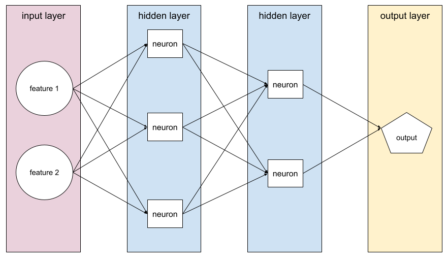
Each neuron in a neural network connects to all of the nodes in the next layer. For example, in the preceding diagram, notice that each of the three neurons in the first hidden layer separately connect to both of the two neurons in the second hidden layer.
Neural networks implemented on computers are sometimes called artificial neural networks to differentiate them from neural networks found in brains and other nervous systems.
Some neural networks can mimic extremely complex nonlinear relationships between different features and the label.
See also convolutional neural network and recurrent neural network .
See Neural networks in Machine Learning Crash Course for more information.
нейрон
In machine learning, a distinct unit within a hidden layer of a neural network . Each neuron performs the following two-step action:
- Calculates the weighted sum of input values multiplied by their corresponding weights.
- Passes the weighted sum as input to an activation function .
A neuron in the first hidden layer accepts inputs from the feature values in the input layer . A neuron in any hidden layer beyond the first accepts inputs from the neurons in the preceding hidden layer. For example, a neuron in the second hidden layer accepts inputs from the neurons in the first hidden layer.
The following illustration highlights two neurons and their inputs.
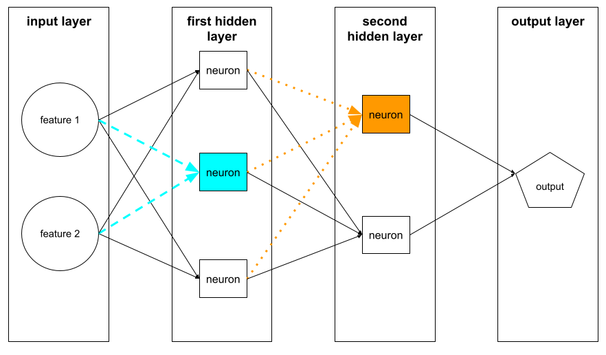
A neuron in a neural network mimics the behavior of neurons in brains and other parts of nervous systems.
N-gram
An ordered sequence of N words. For example, truly madly is a 2-gram. Because order is relevant, madly truly is a different 2-gram than truly madly .
| Н | Name(s) for this kind of N-gram | Примеры |
|---|---|---|
| 2 | bigram or 2-gram | to go, go to, eat lunch, eat dinner |
| 3 | trigram or 3-gram | ate too much, happily ever after, the bell tolls |
| 4 | 4-gram | walk in the park, dust in the wind, the boy ate lentils |
Many natural language understanding models rely on N-grams to predict the next word that the user will type or say. For example, suppose a user typed happily ever . An NLU model based on trigrams would likely predict that the user will next type the word after .
Contrast N-grams with bag of words , which are unordered sets of words.
See Large language models in Machine Learning Crash Course for more information.
НЛП
Abbreviation for natural language processing .
НЛУ
Abbreviation for natural language understanding .
node (decision tree)
In a decision tree , any condition or leaf .
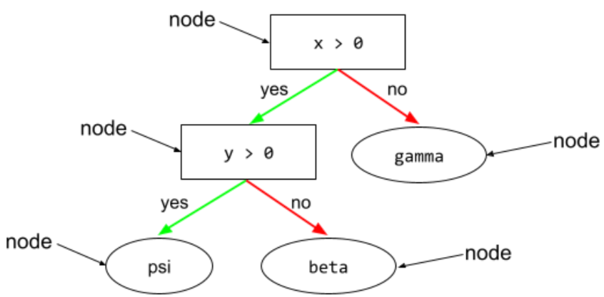
See Decision Trees in the Decision Forests course for more information.
node (neural network)
A neuron in a hidden layer .
See Neural Networks in Machine Learning Crash Course for more information.
node (TensorFlow graph)
An operation in a TensorFlow graph .
шум
Broadly speaking, anything that obscures the signal in a dataset. Noise can be introduced into data in a variety of ways. For example:
- Human raters make mistakes in labeling.
- Humans and instruments mis-record or omit feature values.
non-binary condition
A condition containing more than two possible outcomes. For example, the following non-binary condition contains three possible outcomes:
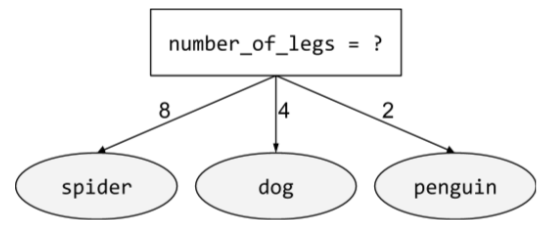
See Types of conditions in the Decision Forests course for more information.
недетерминированный
A system that is not guaranteed to return the same output for a given input. LLMs are generally nondeterministic; that is, LLMs typically generate different responses to the same prompt .
Nondeterministic systems are generally much harder to test than deterministic systems.
See also probabilistic .
нелинейный
A relationship between two or more variables that can't be represented solely through addition and multiplication. A linear relationship can be represented as a line; a nonlinear relationship can't be represented as a line. For example, consider two models that each relate a single feature to a single label. The model on the left is linear and the model on the right is nonlinear:
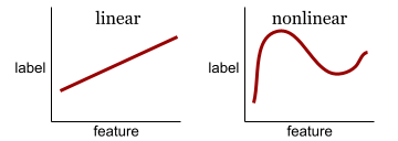
See Neural networks: Nodes and hidden layers in Machine Learning Crash Course to experiment with different kinds of nonlinear functions.
non-response bias
See selection bias .
nonstationarity
A feature whose values change across one or more dimensions, usually time. For example, consider the following examples of nonstationarity:
- The number of swimsuits sold at a particular store varies with the season.
- The quantity of a particular fruit harvested in a particular region is zero for much of the year but large for a brief period.
- Due to climate change, annual mean temperatures are shifting.
Contrast with stationarity .
no one right answer (NORA)
A prompt having multiple correct responses . For example, the following prompt has no one right answer:
Tell me a funny joke about elephants.
Evaluating the responses to no one right answer prompts is usually far more subjective than evaluating prompts with one right answer . For example, evaluating an elephant joke requires a systematic way to determine how funny the joke is.
НОРА
Abbreviation for no one right answer .
нормализация
Broadly speaking, the process of converting a variable's actual range of values into a standard range of values, such as:
- -1 to +1
- от 0 до 1
- Z-scores (roughly, -3 to +3)
For example, suppose the actual range of values of a certain feature is 800 to 2,400. As part of feature engineering , you could normalize the actual values down to a standard range, such as -1 to +1.
Normalization is a common task in feature engineering . Models usually train faster (and produce better predictions) when every numerical feature in the feature vector has roughly the same range.
See also Z-score normalization .
See Numerical Data: Normalization in Machine Learning Crash Course for more information.
Блокнот LM
A Gemini-based tool that enables users to upload documents and then use prompts to ask questions about, summarize, or organize those documents. For example, an author could upload several short stories and ask Notebook LM to find their common themes or to identify which one would make the best movie.
novelty detection
The process of determining whether a new (novel) example comes from the same distribution as the training set . In other words, after training on the training set, novelty detection determines whether a new example (during inference or during additional training) is an outlier .
Contrast with outlier detection .
числовые данные
Features represented as integers or real-valued numbers. For example, a house valuation model would probably represent the size of a house (in square feet or square meters) as numerical data. Representing a feature as numerical data indicates that the feature's values have a mathematical relationship to the label. That is, the number of square meters in a house probably has some mathematical relationship to the value of the house.
Not all integer data should be represented as numerical data. For example, postal codes in some parts of the world are integers; however, integer postal codes shouldn't be represented as numerical data in models. That's because a postal code of 20000 is not twice (or half) as potent as a postal code of 10000. Furthermore, although different postal codes do correlate to different real estate values, we can't assume that real estate values at postal code 20000 are twice as valuable as real estate values at postal code 10000. Postal codes should be represented as categorical data instead.
Numerical features are sometimes called continuous features .
See Working with numerical data in Machine Learning Crash Course for more information.
NumPy
An open-source math library that provides efficient array operations in Python. pandas is built on NumPy.
О
цель
A metric that your algorithm is trying to optimize.
целевая функция
The mathematical formula or metric that a model aims to optimize. For example, the objective function for linear regression is usually Mean Squared Loss . Therefore, when training a linear regression model, training aims to minimize Mean Squared Loss.
In some cases, the goal is to maximize the objective function. For example, if the objective function is accuracy, the goal is to maximize accuracy.
See also loss .
oblique condition
In a decision tree , a condition that involves more than one feature . For example, if height and width are both features, then the following is an oblique condition:
height > width
Contrast with axis-aligned condition .
See Types of conditions in the Decision Forests course for more information.
наблюдать
A stage in the agentic loop in which the agent examines or evaluates some aspect of the agent's progress. For example, suppose that the act stage generates some code. Consequently, the observe stage might run tests on the generated code.
офлайн
Synonym for static .
offline inference
The process of a model generating a batch of predictions and then caching (saving) those predictions. Apps can then access the inferred prediction from the cache rather than rerunning the model.
For example, consider a model that generates local weather forecasts (predictions) once every four hours. After each model run, the system caches all the local weather forecasts. Weather apps retrieve the forecasts from the cache.
Offline inference is also called static inference .
Contrast with online inference . See Production ML systems: Static versus dynamic inference in Machine Learning Crash Course for more information.
one-hot encoding
Representing categorical data as a vector in which:
- One element is set to 1.
- All other elements are set to 0.
One-hot encoding is commonly used to represent strings or identifiers that have a finite set of possible values. For example, suppose a certain categorical feature named Scandinavia has five possible values:
- "Дания"
- "Швеция"
- "Норвегия"
- "Финляндия"
- "Исландия"
One-hot encoding could represent each of the five values as follows:
| Страна | Вектор | ||||
|---|---|---|---|---|---|
| "Дания" | 1 | 0 | 0 | 0 | 0 |
| "Швеция" | 0 | 1 | 0 | 0 | 0 |
| "Норвегия" | 0 | 0 | 1 | 0 | 0 |
| "Финляндия" | 0 | 0 | 0 | 1 | 0 |
| "Исландия" | 0 | 0 | 0 | 0 | 1 |
Thanks to one-hot encoding, a model can learn different connections based on each of the five countries.
Representing a feature as numerical data is an alternative to one-hot encoding. Unfortunately, representing the Scandinavian countries numerically is not a good choice. For example, consider the following numeric representation:
- "Denmark" is 0
- "Sweden" is 1
- "Norway" is 2
- "Finland" is 3
- "Iceland" is 4
With numeric encoding, a model would interpret the raw numbers mathematically and would try to train on those numbers. However, Iceland isn't actually twice as much (or half as much) of something as Norway, so the model would come to some strange conclusions.
See Categorical data: Vocabulary and one-hot encoding in Machine Learning Crash Course for more information.
one right answer (ORA)
A prompt having a single correct response . For example, consider the following prompt:
True or false: Saturn is bigger than Mars.
The only correct response is true .
Contrast with no one right answer .
one-shot learning
A machine learning approach, often used for object classification, designed to learn effective classification model from a single training example.
See also few-shot learning and zero-shot learning .
one-shot prompting
A prompt that contains one example demonstrating how the large language model should respond. For example, the following prompt contains one example showing a large language model how it should answer a query.
| Parts of one prompt | Примечания |
|---|---|
| What is the official currency of the specified country? | The question you want the LLM to answer. |
| France: EUR | One example. |
| Индия: | The actual query. |
Compare and contrast one-shot prompting with the following terms:
one-vs.-all
Given a classification problem with N classes, a solution consisting of N separate binary classification model—one binary classification model for each possible outcome. For example, given a model that classifies examples as animal, vegetable, or mineral, a one-vs.-all solution would provide the following three separate binary classification models:
- animal versus not animal
- vegetable versus not vegetable
- mineral versus not mineral
онлайн
Synonym for dynamic .
online inference
Generating predictions on demand. For example, suppose an app passes input to a model and issues a request for a prediction. A system using online inference responds to the request by running the model (and returning the prediction to the app).
Contrast with offline inference .
See Production ML systems: Static versus dynamic inference in Machine Learning Crash Course for more information.
operation (op)
In TensorFlow, any procedure that creates, manipulates, or destroys a Tensor . For example, a matrix multiply is an operation that takes two Tensors as input and generates one Tensor as output.
Optax
A gradient processing and optimization library for JAX . Optax facilitates research by providing building blocks that can be recombined in custom ways to optimize parametric models such as deep neural networks. Other goals include:
- Providing readable, well-tested, efficient implementations of core components.
- Improving productivity by making it possible to combine low level ingredients into custom optimizers (or other gradient processing components).
- Accelerating adoption of new ideas by making it easy for anyone to contribute.
оптимизатор
A specific implementation of the gradient descent algorithm. Popular optimizers include:
- AdaGrad , which stands for ADAptive GRADient descent.
- Adam, which stands for ADAptive with Momentum.
ОРА
Abbreviation for one right answer .
out-group homogeneity bias
The tendency to see out-group members as more alike than in-group members when comparing attitudes, values, personality traits, and other characteristics. In-group refers to people you interact with regularly; out-group refers to people you don't interact with regularly. If you create a dataset by asking people to provide attributes about out-groups, those attributes may be less nuanced and more stereotyped than attributes that participants list for people in their in-group.
For example, Lilliputians might describe the houses of other Lilliputians in great detail, citing small differences in architectural styles, windows, doors, and sizes. However, the same Lilliputians might simply declare that Brobdingnagians all live in identical houses.
Out-group homogeneity bias is a form of group attribution bias .
See also in-group bias .
обнаружение выбросов
The process of identifying outliers in a training set .
Contrast with novelty detection .
выбросы
Values distant from most other values. In machine learning, any of the following are outliers:
- Input data whose values are more than roughly 3 standard deviations from the mean.
- Weights with high absolute values.
- Predicted values relatively far away from the actual values.
For example, suppose that widget-price is a feature of a certain model. Assume that the mean widget-price is 7 Euros with a standard deviation of 1 Euro. Examples containing a widget-price of 12 Euros or 2 Euros would therefore be considered outliers because each of those prices is five standard deviations from the mean.
Outliers are often caused by typos or other input mistakes. In other cases, outliers aren't mistakes; after all, values five standard deviations away from the mean are rare but hardly impossible.
Outliers often cause problems in model training. Clipping is one way of managing outliers.
See Working with numerical data in Machine Learning Crash Course for more information.
out-of-bag evaluation (OOB evaluation)
A mechanism for evaluating the quality of a decision forest by testing each decision tree against the examples not used during training of that decision tree. For example, in the following diagram, notice that the system trains each decision tree on about two-thirds of the examples and then evaluates against the remaining one-third of the examples.
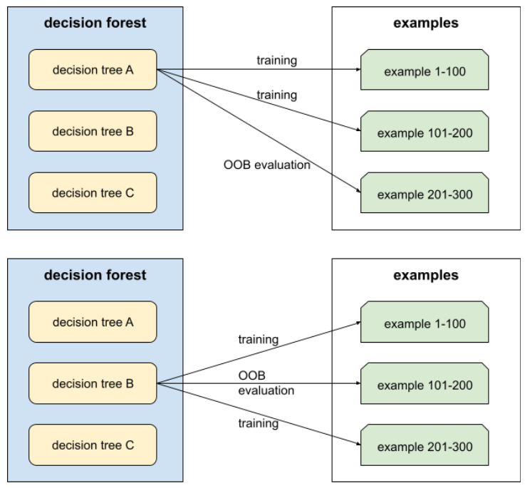
Out-of-bag evaluation is a computationally efficient and conservative approximation of the cross-validation mechanism. In cross-validation, one model is trained for each cross-validation round (for example, 10 models are trained in a 10-fold cross-validation). With OOB evaluation, a single model is trained. Because bagging withholds some data from each tree during training, OOB evaluation can use that data to approximate cross-validation.
See Out-of-bag evaluation in the Decision Forests course for more information.
output layer
The "final" layer of a neural network. The output layer contains the prediction.
The following illustration shows a small deep neural network with an input layer, two hidden layers, and an output layer:
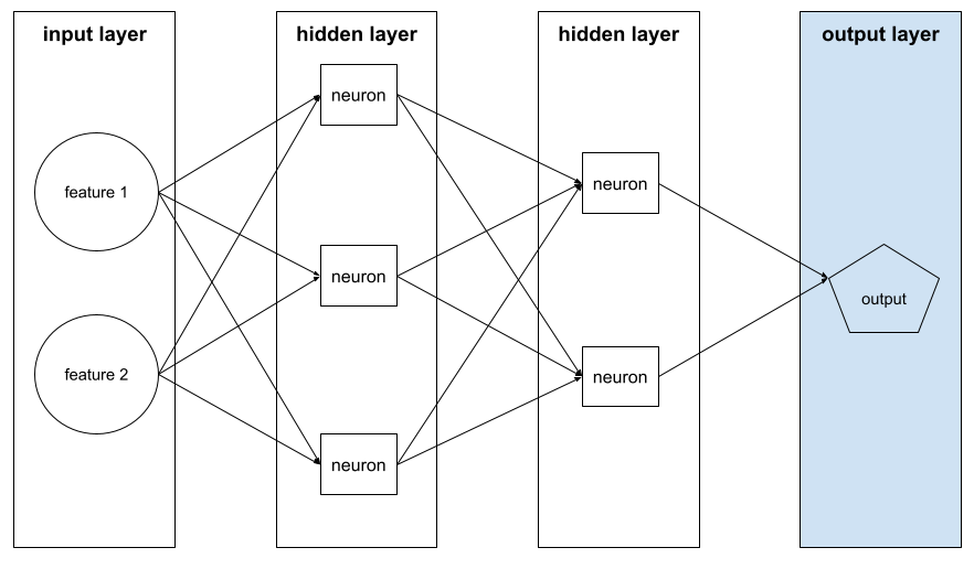
overfitting
Creating a model that matches the training data so closely that the model fails to make correct predictions on new data.
Regularization can reduce overfitting. Training on a large and diverse training set can also reduce overfitting.
See Overfitting in Machine Learning Crash Course for more information.
oversampling
Reusing the examples of a minority class in a class-imbalanced dataset in order to create a more balanced training set .
For example, consider a binary classification problem in which the ratio of the majority class to the minority class is 5,000:1. If the dataset contains a million examples, then the dataset contains only about 200 examples of the minority class, which might be too few examples for effective training. To overcome this deficiency, you might oversample (reuse) those 200 examples multiple times, possibly yielding sufficient examples for useful training.
You need to be careful about over overfitting when oversampling.
Contrast with undersampling .
П
packed data
An approach for storing data more efficiently.
Packed data stores data either by using a compressed format or in some other way that allows it to be accessed more efficiently. Packed data minimizes the amount of memory and computation required to access it, leading to faster training and more efficient model inference.
Packed data is often used with other techniques, such as data augmentation and regularization , further improving the performance of models .
Ладонь
Abbreviation for Pathways Language Model .
панды
A column-oriented data analysis API built on top of numpy . Many machine learning frameworks, including TensorFlow, support pandas data structures as inputs. See the pandas documentation for details.
параметр
The weights and biases that a model learns during training . For example, in a linear regression model, the parameters consist of the bias ( b ) and all the weights ( w 1 , w 2 , and so on) in the following formula:
In contrast, hyperparameters are the values that you (or a hyperparameter tuning service) supply to the model. For example, learning rate is a hyperparameter.
parameter-efficient tuning
A set of techniques to fine-tune a large pre-trained language model (PLM) more efficiently than full fine-tuning . Parameter-efficient tuning typically fine-tunes far fewer parameters than full fine-tuning, yet generally produces a large language model that performs as well (or almost as well) as a large language model built from full fine-tuning.
Compare and contrast parameter-efficient tuning with:
Parameter-efficient tuning is also known as parameter-efficient fine-tuning .
Parameter Server (PS)
A job that keeps track of a model's parameters in a distributed setting.
parameter update
The operation of adjusting a model's parameters during training, typically within a single iteration of gradient descent .
partial derivative
A derivative in which all but one of the variables is considered a constant. For example, the partial derivative of f(x, y) with respect to x is the derivative of f considered as a function of x alone (that is, keeping y constant). The partial derivative of f with respect to x focuses only on how x is changing and ignores all other variables in the equation.
participation bias
Synonym for non-response bias. See selection bias .
partitioning strategy
The algorithm by which variables are divided across parameter servers .
pass at k (pass@k)
A metric to determine the quality of code (for example, Python) that a large language model generates. More specifically, pass at k tells you the likelihood that at least one generated block of code out of k generated blocks of code will pass all of its unit tests.
Large language models often struggle to generate good code for complex programming problems. Software engineers adapt to this problem by prompting the large language model to generate multiple ( k ) solutions for the same problem. Then, software engineers test each of the solutions against unit tests. The calculation of pass at k depends on the outcome of the unit tests:
- If one or more of those solutions pass the unit test, then the LLM Passes that code generation challenge.
- If none of the solutions pass the unit test, then the LLM Fails that code generation challenge.
The formula for pass at k is as follows:
\[\text{pass at k} = \frac{\text{total number of passes}} {\text{total number of challenges}}\]
In general, higher values of k produce higher pass at k scores; however, higher values of k require more large language model and unit testing resources.
Pathways Language Model (PaLM)
An older model and predecessor to Gemini models .
Пакс
A programming framework designed for training large-scale neural network models so large that they span multiple TPU accelerator chip slices or pods .
Pax is built on Flax , which is built on JAX .
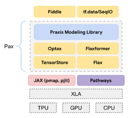
перцептрон
A system (either hardware or software) that takes in one or more input values, runs a function on the weighted sum of the inputs, and computes a single output value. In machine learning, the function is typically nonlinear, such as ReLU , sigmoid , or tanh . For example, the following perceptron relies on the sigmoid function to process three input values:
In the following illustration, the perceptron takes three inputs, each of which is itself modified by a weight before entering the perceptron:

Perceptrons are the neurons in neural networks .
производительность
Overloaded term with the following meanings:
- The standard meaning within software engineering. Namely: How fast (or efficiently) does this piece of software run?
- The meaning within machine learning. Here, performance answers the following question: How correct is this model ? That is, how good are the model's predictions?
permutation variable importances
A type of variable importance that evaluates the increase in the prediction error of a model after permuting the feature's values. Permutation variable importance is a model-independent metric.
недоумение
One measure of how well a model is accomplishing its task. For example, suppose your task is to read the first few letters of a word a user is typing on a phone keyboard, and to offer a list of possible completion words. Perplexity, P, for this task is approximately the number of guesses you need to offer in order for your list to contain the actual word the user is trying to type.
Perplexity is related to cross-entropy as follows:
конвейер
The infrastructure surrounding a machine learning algorithm. A pipeline includes gathering the data, putting the data into training data files, training one or more models, and exporting the models to production.
See ML pipelines in the Managing ML Projects course for more information.
трубопроводная
A form of model parallelism in which a model's processing is divided into consecutive stages and each stage is executed on a different device. While a stage is processing one batch, the preceding stage can work on the next batch.
See also staged training .
pjit
A JAX function that splits code to run across multiple accelerator chips . The user passes a function to pjit, which returns a function that has the equivalent semantics but is compiled into an XLA computation that runs across multiple devices (such as GPUs or TPU cores).
pjit enables users to shard computations without rewriting them by using the SPMD partitioner.
As of March 2023, pjit has been merged with jit . Refer to Distributed arrays and automatic parallelization for more details.
plan-and-solve
An agentic strategy where the model first drafts an explicit, multi-step plan before attempting to execute any actions.
ПЛМ
Abbreviation for pre-trained language model .
плагин
A standardized, modular tool that can be easily attached to an agent to extend its capabilities. For example, a GitHub plugin enables agents to perform actions like reading GitHub issues and creating pull requests.
pmap
A JAX function that executes copies of an input function on multiple underlying hardware devices (CPUs, GPUs, or TPUs ), with different input values. pmap relies on SPMD .
политика
In reinforcement learning, an agent's probabilistic mapping from states to actions .
объединение
Reducing a matrix (or matrixes) created by an earlier convolutional layer to a smaller matrix. Pooling usually involves taking either the maximum or average value across the pooled area. For example, suppose we have the following 3x3 matrix:
![The 3x3 matrix [[5,3,1], [8,2,5], [9,4,3]].](https://developers.google.com/static/machine-learning/glossary/images/PoolingStart.svg?authuser=1&hl=ru)
A pooling operation, just like a convolutional operation, divides that matrix into slices and then slides that convolutional operation by strides . For example, suppose the pooling operation divides the convolutional matrix into 2x2 slices with a 1x1 stride. As the following diagram illustrates, four pooling operations take place. Imagine that each pooling operation picks the maximum value of the four in that slice:
![The input matrix is 3x3 with the values: [[5,3,1], [8,2,5], [9,4,3]].
The top-left 2x2 submatrix of the input matrix is [[5,3], [8,2]], so
the top-left pooling operation yields the value 8 (which is the
maximum of 5, 3, 8, and 2). The top-right 2x2 submatrix of the input
matrix is [[3,1], [2,5]], so the top-right pooling operation yields
the value 5. The bottom-left 2x2 submatrix of the input matrix is
[[8,2], [9,4]], so the bottom-left pooling operation yields the value
9. The bottom-right 2x2 submatrix of the input matrix is
[[2,5], [4,3]], so the bottom-right pooling operation yields the value
5. In summary, the pooling operation yields the 2x2 matrix
[[8,5], [9,5]].](https://developers.google.com/static/machine-learning/glossary/images/PoolingConvolution.svg?authuser=1&hl=ru)
Pooling helps enforce translational invariance in the input matrix.
Pooling for vision applications is known more formally as spatial pooling . Time-series applications usually refer to pooling as temporal pooling . Less formally, pooling is often called subsampling or downsampling .
positional encoding
A technique to add information about the position of a token in a sequence to the token's embedding. Transformer models use positional encoding to better understand the relationship between different parts of the sequence.
A common implementation of positional encoding uses a sinusoidal function. (Specifically, the frequency and amplitude of the sinusoidal function are determined by the position of the token in the sequence.) This technique enables a Transformer model to learn to attend to different parts of the sequence based on their position.
positive class
The class you are testing for.
For example, the positive class in a cancer model might be "tumor." The positive class in an email classification model might be "spam."
Contrast with negative class .
post-processing
Adjusting the output of a model after the model has been run. Post-processing can be used to enforce fairness constraints without modifying models themselves.
For example, one might apply post-processing to a binary classification model by setting a classification threshold such that equality of opportunity is maintained for some attribute by checking that the true positive rate is the same for all values of that attribute.
post-trained model
Loosely-defined term that typically refers to a pre-trained model that has gone through some post-processing, such as one or more of the following:
PR AUC (area under the PR curve)
Area under the interpolated precision-recall curve , obtained by plotting (recall, precision) points for different values of the classification threshold .
Практика
A core, high-performance ML library of Pax . Praxis is often called the "Layer library".
Praxis contains not just the definitions for the Layer class, but most of its supporting components as well, including:
- data inputs
- configuration libraries (HParam and Fiddle )
- оптимизаторы
Praxis provides the definitions for the Model class.
точность
A metric for classification models that answers the following question:
When the model predicted the positive class , what percentage of the predictions were correct?
Here is the formula:
где:
- true positive means the model correctly predicted the positive class.
- false positive means the model mistakenly predicted the positive class.
For example, suppose a model made 200 positive predictions. Of these 200 positive predictions:
- 150 were true positives.
- 50 were false positives.
В этом случае:
Contrast with accuracy and recall .
See Classification: Accuracy, recall, precision and related metrics in Machine Learning Crash Course for more information.
precision at k (precision@k)
A metric for evaluating a ranked (ordered) list of items. Precision at k identifies the fraction of the first k items in that list that are "relevant." That is:
\[\text{precision at k} = \frac{\text{relevant items in first k items of the list}} {\text{k}}\]
The value of k must be less than or equal to the length of the returned list. Note that the length of the returned list is not part of the calculation.
Relevance is often subjective; even expert human evaluators often disagree on which items are relevant.
Сравните с:
precision-recall curve
A curve of precision versus recall at different classification thresholds .
прогноз
A model's output. For example:
- The prediction of a binary classification model is either the positive class or the negative class.
- The prediction of a multi-class classification model is one class.
- The prediction of a linear regression model is a number.
prediction bias
A value indicating how far apart the average of predictions is from the average of labels in the dataset.
Not to be confused with the bias term in machine learning models or with bias in ethics and fairness .
predictive ML
Any standard ("classic") machine learning system.
The term predictive ML doesn't have a formal definition. Rather, the term distinguishes a category of ML systems not based on generative AI .
predictive parity
A fairness metric that checks whether, for a given classification model , the precision rates are equivalent for subgroups under consideration.
For example, a model that predicts college acceptance would satisfy predictive parity for nationality if its precision rate is the same for Lilliputians and Brobdingnagians.
Predictive parity is sometime also called predictive rate parity .
See "Fairness Definitions Explained" (section 3.2.1) for a more detailed discussion of predictive parity.
predictive rate parity
Another name for predictive parity .
предварительная обработка
Processing data before it's used to train a model. Preprocessing could be as simple as removing words from an English text corpus that don't occur in the English dictionary, or could be as complex as re-expressing data points in a way that eliminates as many attributes that are correlated with sensitive attributes as possible. Preprocessing can help satisfy fairness constraints .pre-trained model
Although this term could refer to any trained model or trained embedding vector , pre-trained model now typically refers to a trained large language model or other form of trained generative AI model.
See also base model and foundation model .
pre-training
The initial training of a model on a large dataset . Some pre-trained models are clumsy giants and must typically be refined through additional training. For example, ML experts might pre-train a large language model on a vast text dataset, such as all the English pages in Wikipedia. Following pre-training, the resulting model might be further refined through any of the following techniques:
prior belief
What you believe about the data before you begin training on it. For example, L 2 regularization relies on a prior belief that weights should be small and normally distributed around zero.
Про
A Gemini model with fewer parameters than Ultra but more parameters than Nano . See Gemini Pro for details.
вероятностный
In general, any situation in which decisions are made based on likelihoods or odds. LLMs are probabilistic systems, generating the next word or sentence in a response based on probabilities.
If the temperature is relatively low, an LLM will choose words or sentences having high probabilities. If the temperature is relatively high, an LLM will be more "creative," sometimes choosing words or sentences having lower probabilities.
probabilistic regression model
A regression model that uses not only the weights for each feature , but also the uncertainty of those weights. A probabilistic regression model generates a prediction and the uncertainty of that prediction. For example, a probabilistic regression model might yield a prediction of 325 with a standard deviation of 12. For more information about probabilistic regression models, see this Colab on tensorflow.org .
функция плотности вероятности
A function that identifies the frequency of data samples having exactly a particular value. When a dataset's values are continuous floating-point numbers, exact matches rarely occur. However, integrating a probability density function from value x to value y yields the expected frequency of data samples between x and y .
For example, consider a normal distribution having a mean of 200 and a standard deviation of 30. To determine the expected frequency of data samples falling within the range 211.4 to 218.7, you can integrate the probability density function for a normal distribution from 211.4 to 218.7.
процедурная память
In agents , the knowledge of how to do something. For example, an agent might develop a procedural memory of how to search the web and then display the top three sites.
быстрый
Any text entered as input to a large language model to condition the model to behave in a certain way. Prompts can be as short as a phrase or arbitrarily long (for example, the entire text of a novel). Prompts fall into multiple categories, including those shown in the following table:
| Prompt category | Пример | Примечания |
|---|---|---|
| Вопрос | How fast can a pigeon fly? | |
| Инструкция | Write a funny poem about arbitrage. | A prompt that asks the large language model to do something. |
| Пример | Translate Markdown code to HTML. For example: Markdown: * list item HTML: <ul> <li>list item</li> </ul> | The first sentence in this example prompt is an instruction. The remainder of the prompt is the example. |
| Роль | Explain why gradient descent is used in machine learning training to a PhD in Physics. | The first part of the sentence is an instruction; the phrase "to a PhD in Physics" is the role portion. |
| Partial input for the model to complete | The Prime Minister of the United Kingdom lives at | A partial input prompt can either end abruptly (as this example does) or end with an underscore. |
A generative AI model can respond to a prompt with text, code, images, embeddings , videos…almost anything.
prompt-based learning
A capability of certain models that enables them to adapt their behavior in response to arbitrary text input ( prompts ). In a typical prompt-based learning paradigm, a large language model responds to a prompt by generating text. For example, suppose a user enters the following prompt:
Summarize Newton's Third Law of Motion.
A model capable of prompt-based learning isn't specifically trained to answer the previous prompt. Rather, the model "knows" a lot of facts about physics, a lot about general language rules, and a lot about what constitutes generally useful answers. That knowledge is sufficient to provide a (hopefully) useful answer. Additional human feedback ("That answer was too complicated." or "What's a reaction?") enables some prompt-based learning systems to gradually improve the usefulness of their answers.
prompt chaining
Using the output of one prompt as the input to another prompt. Least-to-most prompting is a popular form of prompt chaining.
prompt design
Synonym for prompt engineering .
оперативное проектирование
The art of creating prompts that elicit the desired responses from a large language model . Humans perform prompt engineering. Writing well-structured prompts is an essential part of ensuring useful responses from a large language model. Prompt engineering depends on many factors, including:
- The dataset used to pre-train and possibly fine-tune the large language model.
- The temperature and other decoding parameters that the model uses to generate responses.
Prompt design is a synonym for prompt engineering.
See Introduction to prompt design for more details on writing helpful prompts.
prompt set
A group of prompts for evaluating a large language model . For example, the following illustration shows a prompt set consisting of three prompts:
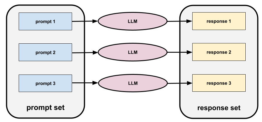
Good prompt sets consist of a sufficiently "wide" collection of prompts to thoroughly evaluate the safety and helpfulness of a large language model.
See also response set .
prompt tuning
A parameter efficient tuning mechanism that learns a "prefix" that the system prepends to the actual prompt .
One variation of prompt tuning—sometimes called prefix tuning —is to prepend the prefix at every layer . In contrast, most prompt tuning only adds a prefix to the input layer .
происхождение
Data detailing how a piece of digital media content was created or changed.
proxy (sensitive attributes)
An attribute used as a stand-in for a sensitive attribute . For example, an individual's postal code might be used as a proxy for their income, race, or ethnicity.proxy labels
Data used to approximate labels not directly available in a dataset.
For example, suppose you must train a model to predict employee stress level. Your dataset contains a lot of predictive features but doesn't contain a label named stress level. Undaunted, you pick "workplace accidents" as a proxy label for stress level. After all, employees under high stress get into more accidents than calm employees. Or do they? Maybe workplace accidents actually rise and fall for multiple reasons.
As a second example, suppose you want is it raining? to be a Boolean label for your dataset, but your dataset doesn't contain rain data. If photographs are available, you might establish pictures of people carrying umbrellas as a proxy label for is it raining? Is that a good proxy label? Possibly, but people in some cultures may be more likely to carry umbrellas to protect against sun than the rain.
Proxy labels are often imperfect. When possible, choose actual labels over proxy labels. That said, when an actual label is absent, pick the proxy label very carefully, choosing the least horrible proxy label candidate.
See Datasets: Labels in Machine Learning Crash Course for more information.
чистая функция
A function whose outputs are based only on its inputs, and that has no side effects. Specifically, a pure function doesn't use or change any global state, such as the contents of a file or the value of a variable outside the function.
Pure functions can be used to create thread-safe code, which is beneficial when sharding model code across multiple accelerator chips .
JAX's function transformation methods require that the input functions are pure functions.
В
Q-function
In reinforcement learning , the function that predicts the expected return from taking an action in a state and then following a given policy .
Q-function is also known as state-action value function .
Q-обучение
In reinforcement learning , an algorithm that allows an agent to learn the optimal Q-function of a Markov decision process by applying the Bellman equation . The Markov decision process models an environment .
quantile
Each bucket in quantile bucketing .
quantile bucketing
Distributing a feature's values into buckets so that each bucket contains the same (or almost the same) number of examples. For example, the following figure divides 44 points into 4 buckets, each of which contains 11 points. In order for each bucket in the figure to contain the same number of points, some buckets span a different width of x-values.

See Numerical data: Binning in Machine Learning Crash Course for more information.
квантование
Overloaded term that could be used in any of the following ways:
- Implementing quantile bucketing on a particular feature .
- Transforming data into zeroes and ones for quicker storing, training, and inferring. As Boolean data is more robust to noise and errors than other formats, quantization can improve model correctness. Quantization techniques include rounding, truncating, and binning .
Reducing the number of bits used to store a model's parameters . For example, suppose a model's parameters are stored as 32-bit floating-point numbers. Quantization converts those parameters from 32 bits down to 4, 8, or 16 bits. Quantization reduces the following:
- Compute, memory, disk, and network usage
- Time to infer a predication
- Потребление электроэнергии
However, quantization sometimes decreases the correctness of a model's predictions.
очередь
A TensorFlow Operation that implements a queue data structure. Typically used in I/O.
Р
ТРЯПКА
Abbreviation for retrieval-augmented generation .
random forest
An ensemble of decision trees in which each decision tree is trained with a specific random noise, such as bagging .
Random forests are a type of decision forest .
See Random Forest in the Decision Forests course for more information.
random policy
In reinforcement learning , a policy that chooses an action at random.
rank (ordinality)
The ordinal position of a class in a machine learning problem that categorizes classes from highest to lowest. For example, a behavior ranking system could rank a dog's rewards from highest (a steak) to lowest (wilted kale).
rank (Tensor)
The number of dimensions in a Tensor . For example, a scalar has rank 0, a vector has rank 1, and a matrix has rank 2.
Not to be confused with rank (ordinality) .
рейтинг
A type of supervised learning whose objective is to order a list of items.
оценщик
A human who provides labels for examples . "Annotator" is another name for rater.
See Categorical data: Common issues in Machine Learning Crash Course for more information.
Reading Comprehension with Commonsense Reasoning Dataset (ReCoRD)
A dataset to evaluate an LLM's ability to perform commonsense reasoning. Each example in the dataset contains three components:
- A paragraph or two from a news article
- A query in which one of the entities explicitly or implicitly identified in the passage is masked .
- The answer (the name of the entity that belongs in the mask)
See ReCoRD for an extensive list of examples.
ReCoRD is a component of the SuperGLUE ensemble.
RealToxicityPrompts
A dataset that contains a set of sentence beginnings that might contain toxic content. Use this dataset to evaluate an LLM's ability to generate non-toxic text to complete the sentence. Typically, you use the Perspective API to determine how well the LLM performed at this task.
See RealToxicityPrompts: Evaluating Neural Toxic Degeneration in Language Models for details.
причина
A stage in the agentic loop in which the agent determines what to do. For example, the agent might determine that a particular API request should be sent.
отзывать
A metric for classification models that answers the following question:
When ground truth was the positive class , what percentage of predictions did the model correctly identify as the positive class?
Here is the formula:
\[\text{Recall} = \frac{\text{true positives}} {\text{true positives} + \text{false negatives}} \]
где:
- true positive means the model correctly predicted the positive class.
- false negative means that the model mistakenly predicted the negative class .
For instance, suppose your model made 200 predictions on examples for which ground truth was the positive class. Of these 200 predictions:
- 180 were true positives.
- 20 were false negatives.
В этом случае:
\[\text{Recall} = \frac{\text{180}} {\text{180} + \text{20}} = 0.9 \]
See Classification: Accuracy, recall, precision and related metrics for more information.
recall at k (recall@k)
A metric for evaluating systems that output a ranked (ordered) list of items. Recall at k identifies the fraction of relevant items in the first k items in that list out of the total number of relevant items returned.
\[\text{recall at k} = \frac{\text{relevant items in first k items of the list}} {\text{total number of relevant items in the list}}\]
Contrast with precision at k .
Recognizing Textual Entailment (RTE)
A dataset for evaluating an LLM's ability to determine whether a hypothesis can be entailed (logically drawn) from a text passage. Each example in an RTE evaluation consists of three parts:
- A passage, typically from news or Wikipedia articles
- A hypothesis
- The correct answer, which is either:
- True, meaning the hypothesis can be entailed from the passage
- False, meaning the hypothesis can't be entailed from the passage
Например:
- Passage: The Euro is the currency of the European Union.
- Hypothesis: France uses the Euro as currency.
- Entailment: True, because France is part of the European Union.
RTE is a component of the SuperGLUE ensemble.
recommendation system
A system that selects for each user a relatively small set of desirable items from a large corpus. For example, a video recommendation system might recommend two videos from a corpus of 100,000 videos, selecting Casablanca and The Philadelphia Story for one user, and Wonder Woman and Black Panther for another. A video recommendation system might base its recommendations on factors such as:
- Movies that similar users have rated or watched.
- Genre, directors, actors, target demographic...
See the Recommendation Systems course for more information.
Записывать
Abbreviation for Reading Comprehension with Commonsense Reasoning Dataset .
Rectified Linear Unit (ReLU)
An activation function with the following behavior:
- If input is negative or zero, then the output is 0.
- If input is positive, then the output is equal to the input.
Например:
- If the input is -3, then the output is 0.
- If the input is +3, then the output is 3.0.
Here is a plot of ReLU:
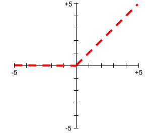
ReLU is a very popular activation function. Despite its simple behavior, ReLU still enables a neural network to learn nonlinear relationships between features and the label .
рекуррентная нейронная сеть
A neural network that is intentionally run multiple times, where parts of each run feed into the next run. Specifically, hidden layers from the previous run provide part of the input to the same hidden layer in the next run. Recurrent neural networks are particularly useful for evaluating sequences, so that the hidden layers can learn from previous runs of the neural network on earlier parts of the sequence.
For example, the following figure shows a recurrent neural network that runs four times. Notice that the values learned in the hidden layers from the first run become part of the input to the same hidden layers in the second run. Similarly, the values learned in the hidden layer on the second run become part of the input to the same hidden layer in the third run. In this way, the recurrent neural network gradually trains and predicts the meaning of the entire sequence rather than just the meaning of individual words.

reference text
An expert's response to a prompt . For example, given the following prompt:
Translate the question "What is your name?" from English to French.
An expert's response might be:
Comment vous appelez-vous?
Various metrics (such as ROUGE ) measure the degree to which the reference text matches an ML model's generated text .
отражение
A strategy for improving the quality of an agentic workflow by examining (reflecting on) a step's output before passing that output to the next step.
The examiner is often the same LLM that generated the response (though it could be a different LLM). How could the same LLM that generated a response be a fair judge of its own response? The "trick" is to put the LLM in a critical (reflective) mindset. This process is analogous to a writer who uses a creative mindset to write a first draft and then switches to a critical mindset to edit it.
For example, imagine an agentic workflow whose first step is to create text for coffee mugs. The prompt for this step might be:
You are a creative. Generate humorous, original text of less than 50 characters suitable for a coffee mug.
Now imagine the following reflective prompt:
You are a coffee drinker. Would you find the preceding response humorous?
The workflow might then only pass text that receives a high reflection score to the next stage.
регрессионная модель
Informally, a model that generates a numerical prediction. (In contrast, a classification model generates a class prediction.) For example, the following are all regression models:
- A model that predicts a certain house's value in Euros, such as 423,000.
- A model that predicts a certain tree's life expectancy in years, such as 23.2.
- A model that predicts the amount of rain in inches that will fall in a certain city over the next six hours, such as 0.18.
Two common types of regression models are:
- Linear regression , which finds the line that best fits label values to features.
- Logistic regression , which generates a probability between 0.0 and 1.0 that a system typically then maps to a class prediction.
Not every model that outputs numerical predictions is a regression model. In some cases, a numeric prediction is really just a classification model that happens to have numeric class names. For example, a model that predicts a numeric postal code is a classification model, not a regression model.
регуляризация
Any mechanism that reduces overfitting . Popular types of regularization include:
- L1- регуляризация
- L2- регуляризация
- dropout regularization
- early stopping (this is not a formal regularization method, but can effectively limit overfitting)
Regularization can also be defined as the penalty on a model's complexity.
See Overfitting: Model complexity in Machine Learning Crash Course for more information.
regularization rate
A number that specifies the relative importance of regularization during training. Raising the regularization rate reduces overfitting but may reduce the model's predictive power. Conversely, reducing or omitting the regularization rate increases overfitting.
See Overfitting: L2 regularization in Machine Learning Crash Course for more information.
reinforcement learning (RL)
A family of algorithms that learn an optimal policy , whose goal is to maximize return when interacting with an environment . For example, the ultimate reward of most games is victory. Reinforcement learning systems can become expert at playing complex games by evaluating sequences of previous game moves that ultimately led to wins and sequences that ultimately led to losses.
Reinforcement Learning from Human Feedback (RLHF)
Using feedback from human raters to improve the quality of a model's responses . For example, an RLHF mechanism can ask users to rate the quality of a model's response with a 👍 or 👎 emoji. The system can then adjust its future responses based on that feedback.
РеЛУ
Abbreviation for Rectified Linear Unit .
replay buffer
In DQN -like algorithms, the memory used by the agent to store state transitions for use in experience replay .
реплика
A copy (or part of) of a training set or model , typically stored on another machine. For example, a system could use the following strategy for implementing data parallelism :
- Place replicas of an existing model on multiple machines.
- Send different subsets of the training set to each replica.
- Aggregate the parameter updates.
A replica can also refer to another copy of an inference server. Increasing the number of replicas increases the number of requests that the system can serve simultaneously but also increases serving costs.
reporting bias
The fact that the frequency with which people write about actions, outcomes, or properties is not a reflection of their real-world frequencies or the degree to which a property is characteristic of a class of individuals. Reporting bias can influence the composition of data that machine learning systems learn from.
For example, in books, the word laughed is more prevalent than breathed . A machine learning model that estimates the relative frequency of laughing and breathing from a book corpus would probably determine that laughing is more common than breathing.
See Fairness: Types of bias in Machine Learning Crash Course for more information.
представление
The process of mapping data to useful features .
re-ranking
The final stage of a recommendation system , during which scored items may be re-graded according to some other (typically, non-ML) algorithm. Re-ranking evaluates the list of items generated by the scoring phase, taking actions such as:
- Eliminating items that the user has already purchased.
- Boosting the score of fresher items.
See Re-ranking in the Recommendation Systems course for more information.
ответ
The text, images, audio, or video that a generative AI model infers . In other words, a prompt is the input to a generative AI model and the response is the output .
response set
The collection of responses a large language model returns to an input prompt set .
retrieval-augmented generation (RAG)
A technique for improving the quality of large language model (LLM) output by grounding it with sources of knowledge retrieved after the model was trained. RAG improves the accuracy of LLM responses by providing the trained LLM with access to information retrieved from trusted knowledge bases or documents.
Common motivations to use retrieval-augmented generation include:
- Increasing the factual accuracy of a model's generated responses.
- Giving the model access to knowledge it was not trained on.
- Changing the knowledge that the model uses.
- Enabling the model to cite sources.
For example, suppose that a chemistry app uses the PaLM API to generate summaries related to user queries. When the app's backend receives a query, the backend:
- Searches for ("retrieves") data that's relevant to the user's query.
- Appends ("augments") the relevant chemistry data to the user's query.
- Instructs the LLM to create a summary based on the appended data.
возвращаться
In reinforcement learning, given a certain policy and a certain state, the return is the sum of all rewards that the agent expects to receive when following the policy from the state to the end of the episode . The agent accounts for the delayed nature of expected rewards by discounting rewards according to the state transitions required to obtain the reward.
Therefore, if the discount factor is \(\gamma\), и \(r_0, \ldots, r_{N}\)denote the rewards until the end of the episode, then the return calculation is as follows:
награда
In reinforcement learning, the numerical result of taking an action in a state , as defined by the environment .
ridge regularization
Synonym for L 2 regularization . The term ridge regularization is more frequently used in pure statistics contexts, whereas L 2 regularization is used more often in machine learning.
РНН
Abbreviation for recurrent neural networks .
ROC (receiver operating characteristic) Curve
A graph of true positive rate versus false positive rate for different classification thresholds in binary classification.
The shape of an ROC curve suggests a binary classification model's ability to separate positive classes from negative classes. Suppose, for example, that a binary classification model perfectly separates all the negative classes from all the positive classes:
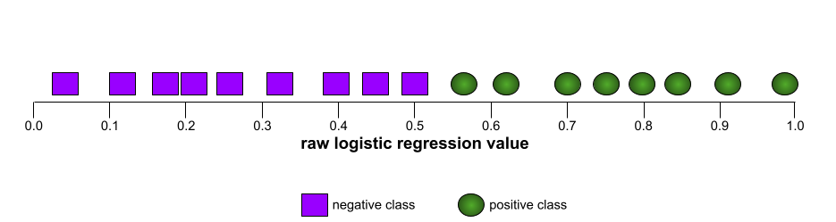
The ROC curve for the preceding model looks as follows:
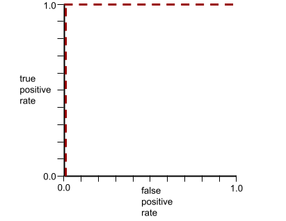
In contrast, the following illustration graphs the raw logistic regression values for a terrible model that can't separate negative classes from positive classes at all:
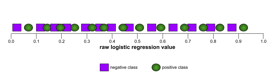
The ROC curve for this model looks as follows:
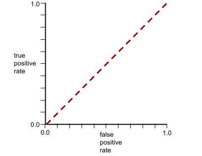
Meanwhile, back in the real world, most binary classification models separate positive and negative classes to some degree, but usually not perfectly. So, a typical ROC curve falls somewhere between the two extremes:
The point on an ROC curve closest to (0.0,1.0) theoretically identifies the ideal classification threshold. However, several other real-world issues influence the selection of the ideal classification threshold. For example, perhaps false negatives cause far more pain than false positives.
A numerical metric called AUC summarizes the ROC curve into a single floating-point value.
role prompting
A prompt , typically beginning with the pronoun you , that tells a generative AI model to pretend to be a certain person or a certain role when generating the response . Role prompting can help a generative AI model get into the right "mindset" in order to generate a more useful response. For example, any of the following role prompts might be appropriate depending on the kind of response you are seeking:
You have a PhD in computer science.
You are a software engineer who enjoys giving patient explanations about Python to new programming students.
You are an action hero with a very particular set of programming skills. Assure me that you will find a particular item in a Python list.
корень
The starting node (the first condition ) in a decision tree . By convention, diagrams put the root at the top of the decision tree. For example:
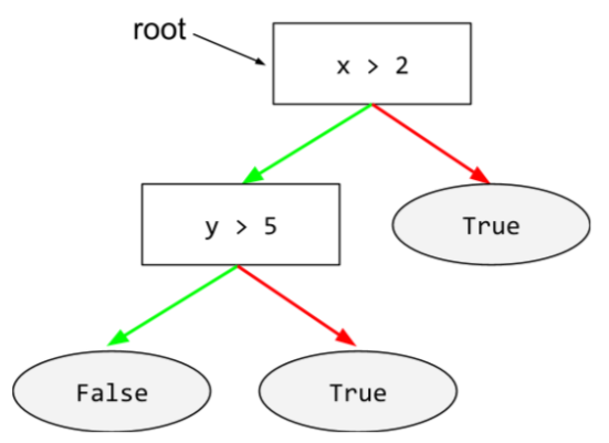
корневой каталог
The directory you specify for hosting subdirectories of the TensorFlow checkpoint and events files of multiple models.
Среднеквадратичная ошибка (RMSE)
The square root of the Mean Squared Error .
rotational invariance
In an image classification problem, an algorithm's ability to successfully classify images even when the orientation of the image changes. For example, the algorithm can still identify a tennis racket whether it is pointing up, sideways, or down. Note that rotational invariance is not always desirable; for example, an upside-down 9 shouldn't be classified as a 9.
See also translational invariance and size invariance .
ROUGE (Recall-Oriented Understudy for Gisting Evaluation)
A family of metrics that evaluate automatic summarization and machine translation models. ROUGE metrics determine the degree to which a reference text overlaps an ML model's generated text . Each member of the ROUGE family measures overlap in a different way. Higher ROUGE scores indicate more similarity between the reference text and generated text than lower ROUGE scores.
Each ROUGE family member typically generates the following metrics:
- Точность
- Отзывать
- Ф 1
For details and examples, see:
ROUGE-L
A member of the ROUGE family focused on the length of the longest common subsequence in the reference text and generated text . The following formulas calculate recall and precision for ROUGE-L:
You can then use F 1 to roll up ROUGE-L recall and ROUGE-L precision into a single metric:
ROUGE-L ignores any newlines in the reference text and generated text, so the longest common subsequence could cross multiple sentences. When the reference text and generated text involve multiple sentences, a variation of ROUGE-L called ROUGE-Lsum is generally a better metric. ROUGE-Lsum determines the longest common subsequence for each sentence in a passage and then calculates the mean of those longest common subsequences.
ROUGE-N
A set of metrics within the ROUGE family that compares the shared N-grams of a certain size in the reference text and generated text . For example:
- ROUGE-1 measures the number of shared tokens in the reference text and generated text.
- ROUGE-2 measures the number of shared bigrams (2-grams) in the reference text and generated text.
- ROUGE-3 measures the number of shared trigrams (3-grams) in the reference text and generated text.
You can use the following formulas to calculate ROUGE-N recall and ROUGE-N precision for any member of the ROUGE-N family:
You can then use F 1 to roll up ROUGE-N recall and ROUGE-N precision into a single metric:
ROUGE-S
A forgiving form of ROUGE-N that enables skip-gram matching. That is, ROUGE-N only counts N-grams that match exactly , but ROUGE-S also counts N-grams separated by one or more words. For example, consider the following:
- reference text : White clouds
- generated text : White billowing clouds
When calculating ROUGE-N, the 2-gram, White clouds doesn't match White billowing clouds . However, when calculating ROUGE-S, White clouds does match White billowing clouds .
router agent
An agent that classifies a user query and then invokes the most appropriate agent to handle it.
R-squared
A regression metric indicating how much variation in a label is due to an individual feature or to a feature set. R-squared is a value between 0 and 1, which you can interpret as follows:
- An R-squared of 0 means that none of a label's variation is due to the feature set.
- An R-squared of 1 means that all of a label's variation is due to the feature set.
- An R-squared between 0 and 1 indicates the extent to which the label's variation can be predicted from a particular feature or the feature set. For example, an R-squared of 0.10 means that 10 percent of the variance in the label is due to the feature set, an R-squared of 0.20 means that 20 percent is due to the feature set, and so on.
R-squared is the square of the Pearson correlation coefficient between the values that a model predicted and ground truth .
РТЭ
Abbreviation for Recognizing Textual Entailment .
С
sampling bias
See selection bias .
sampling with replacement
A method of picking items from a set of candidate items in which the same item can be picked multiple times. The phrase "with replacement" means that after each selection, the selected item is returned to the pool of candidate items. The inverse method, sampling without replacement , means that a candidate item can only be picked once.
For example, consider the following fruit set:
fruit = {kiwi, apple, pear, fig, cherry, lime, mango} Suppose that the system randomly picks fig as the first item. If using sampling with replacement, then the system picks the second item from the following set:
fruit = {kiwi, apple, pear, fig, cherry, lime, mango} Yes, that's the same set as before, so the system could potentially pick fig again.
If using sampling without replacement, once picked, a sample can't be picked again. For example, if the system randomly picks fig as the first sample, then fig can't be picked again. Therefore, the system picks the second sample from the following (reduced) set:
fruit = {kiwi, apple, pear, cherry, lime, mango}SavedModel
The recommended format for saving and recovering TensorFlow models. SavedModel is a language-neutral, recoverable serialization format, which enables higher-level systems and tools to produce, consume, and transform TensorFlow models.
See the Saving and Restoring section of the TensorFlow Programmer's Guide for complete details.
Экономия
A TensorFlow object responsible for saving model checkpoints.
скаляр
A single number or a single string that can be represented as a tensor of rank 0. For example, the following lines of code each create one scalar in TensorFlow:
breed = tf.Variable("poodle", tf.string)
temperature = tf.Variable(27, tf.int16)
precision = tf.Variable(0.982375101275, tf.float64)
масштабирование
Any mathematical transform or technique that shifts the range of a label, a feature value, or both. Some forms of scaling are very useful for transformations like normalization .
Common forms of scaling useful in Machine Learning include:
- linear scaling, which typically uses a combination of subtraction and division to replace the original value with a number between -1 and +1 or between 0 and 1.
- logarithmic scaling, which replaces the original value with its logarithm.
- Z-score normalization , which replaces the original value with a floating-point value representing the number of standard deviations from that feature's mean.
scikit-learn
A popular open-source machine learning platform. See scikit-learn.org .
подсчет очков
The part of a recommendation system that provides a value or ranking for each item produced by the candidate generation phase.
предвзятость отбора
Errors in conclusions drawn from sampled data due to a selection process that generates systematic differences between samples observed in the data and those not observed. The following forms of selection bias exist:
- coverage bias : The population represented in the dataset doesn't match the population that the machine learning model is making predictions about.
- sampling bias : Data is not collected randomly from the target group.
- non-response bias (also called participation bias ): Users from certain groups opt-out of surveys at different rates than users from other groups.
For example, suppose you are creating a machine learning model that predicts people's enjoyment of a movie. To collect training data, you hand out a survey to everyone in the front row of a theater showing the movie. Offhand, this may sound like a reasonable way to gather a dataset; however, this form of data collection may introduce the following forms of selection bias:
- coverage bias: By sampling from a population who chose to see the movie, your model's predictions may not generalize to people who did not already express that level of interest in the movie.
- sampling bias: Rather than randomly sampling from the intended population (all the people at the movie), you sampled only the people in the front row. It is possible that the people sitting in the front row were more interested in the movie than those in other rows.
- non-response bias: In general, people with strong opinions tend to respond to optional surveys more frequently than people with mild opinions. Since the movie survey is optional, the responses are more likely to form a bimodal distribution than a normal (bell-shaped) distribution.
self-attention (also called self-attention layer)
A neural network layer that transforms a sequence of embeddings (for example, token embeddings) into another sequence of embeddings. Each embedding in the output sequence is constructed by integrating information from the elements of the input sequence through an attention mechanism.
The self part of self-attention refers to the sequence attending to itself rather than to some other context. Self-attention is one of the main building blocks for Transformers and uses dictionary lookup terminology, such as "query", "key", and "value".
A self-attention layer starts with a sequence of input representations, one for each word. The input representation for a word can be a simple embedding. For each word in an input sequence, the network scores the relevance of the word to every element in the whole sequence of words. The relevance scores determine how much the word's final representation incorporates the representations of other words.
Например, рассмотрим следующее предложение:
The animal didn't cross the street because it was too tired.
The following illustration (from Transformer: A Novel Neural Network Architecture for Language Understanding ) shows a self-attention layer's attention pattern for the pronoun it , with the darkness of each line indicating how much each word contributes to the representation:
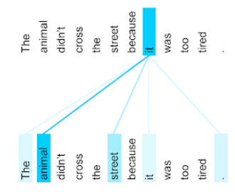
The self-attention layer highlights words that are relevant to "it". In this case, the attention layer has learned to highlight words that it might refer to, assigning the highest weight to animal .
For a sequence of n tokens , self-attention transforms a sequence of embeddings n separate times, once at each position in the sequence.
Refer also to attention and multi-head self-attention .
self-correction
An agent's ability to detect an error in its own output and then try a different approach.
self-supervised learning
A family of techniques for converting an unsupervised machine learning problem into a supervised machine learning problem by creating surrogate labels from unlabeled examples .
Some Transformer -based models such as BERT use self-supervised learning.
Self-supervised training is a semi-supervised learning approach.
self-training
A variant of self-supervised learning that is particularly useful when all of the following conditions are true:
- The ratio of unlabeled examples to labeled examples in the dataset is high.
- This is a classification problem.
Self-training works by iterating over the following two steps until the model stops improving:
- Use supervised machine learning to train a model on the labeled examples.
- Use the model created in Step 1 to generate predictions (labels) on the unlabeled examples, moving those in which there is high confidence into the labeled examples with the predicted label.
Notice that each iteration of Step 2 adds more labeled examples for Step 1 to train on.
semantic memory
The information that an LLM has when training ends. For example, semantic memory includes an excellent knowledge of grammar, vocabulary, and the facts it was explicitly trained on.
Semantic memory does not include information gathered from retrieval-augmented generation .
Contrast semantic memory with episodic memory .
semi-supervised learning
Training a model on data where some of the training examples have labels but others don't. One technique for semi-supervised learning is to infer labels for the unlabeled examples, and then to train on the inferred labels to create a new model. Semi-supervised learning can be useful if labels are expensive to obtain but unlabeled examples are plentiful.
Self-training is one technique for semi-supervised learning.
sensitive attribute
A human attribute that may be given special consideration for legal, ethical, social, or personal reasons.анализ настроений
Using statistical or machine learning algorithms to determine a group's overall attitude—positive or negative—toward a service, product, organization, or topic. For example, using natural language understanding , an algorithm could perform sentiment analysis on the textual feedback from a university course to determine the degree to which students generally liked or disliked the course.
See the Text classification guide for more information.
sequence model
A model whose inputs have a sequential dependence. For example, predicting the next video watched from a sequence of previously watched videos.
sequence-to-sequence task
A task that converts an input sequence of tokens to an output sequence of tokens. For example, two popular kinds of sequence-to-sequence tasks are:
- Переводчики:
- Sample input sequence: "I love you."
- Sample output sequence: "Je t'aime."
- Question answering:
- Sample input sequence: "Do I need my car in New York City?"
- Sample output sequence: "No. Keep your car at home."
подача
The process of making a trained model available to provide predictions through online inference or offline inference .
shape (Tensor)
The number of elements in each dimension of a tensor. The shape is represented as a list of integers. For example, the following two-dimensional tensor has a shape of [3,4]:
[[5, 7, 6, 4],
 [2, 9, 4, 8],
 [3, 6, 5, 1]]
TensorFlow uses row-major (C-style) format to represent the order of dimensions, which is why the shape in TensorFlow is [3,4] rather than [4,3] . In other words, in a two-dimensional TensorFlow Tensor, the shape is [ number of rows , number of columns ] .
A static shape is a tensor shape that is known at compile time.
A dynamic shape is unknown at compile time and is therefore dependent on runtime data. This tensor might be represented with a placeholder dimension in TensorFlow, as in [3, ?] .
осколок
A logical division of the training set or the model . Typically, some process creates shards by dividing the examples or parameters into (usually) equal-sized chunks. Each shard is then assigned to a different machine.
Sharding a model is called model parallelism ; sharding data is called data parallelism .
усадка
A hyperparameter in gradient boosting that controls overfitting . Shrinkage in gradient boosting is analogous to learning rate in gradient descent . Shrinkage is a decimal value between 0.0 and 1.0. A lower shrinkage value reduces overfitting more than a larger shrinkage value.
side-by-side evaluation
Comparing the quality of two models by judging their responses to the same prompt . For example, suppose the following prompt is given to two different models :
Create an image of a cute dog juggling three balls.
In a side-by-side evaluation, a rater would pick which image was "better" (More accurate? More beautiful? Cuter?).
sigmoid function
A mathematical function that "squishes" an input value into a constrained range, typically 0 to 1 or -1 to +1. That is, you can pass any number (two, a million, negative billion, whatever) to a sigmoid and the output will still be in the constrained range. A plot of the sigmoid activation function looks as follows:
The sigmoid function has several uses in machine learning, including:
- Converting the raw output of a logistic regression or multinomial regression model to a probability.
- Acting as an activation function in some neural networks.
similarity measure
In clustering algorithms, the metric used to determine how alike (how similar) any two examples are.
single program / multiple data (SPMD)
A parallelism technique where the same computation is run on different input data in parallel on different devices. The goal of SPMD is to obtain results more quickly. It is the most common style of parallel programming.
size invariance
In an image classification problem, an algorithm's ability to successfully classify images even when the size of the image changes. For example, the algorithm can still identify a cat whether it consumes 2M pixels or 200K pixels. Note that even the best image classification algorithms still have practical limits on size invariance. For example, an algorithm (or human) is unlikely to correctly classify a cat image consuming only 20 pixels.
See also translational invariance and rotational invariance .
See the Clustering course for more information.
эскизирование
In unsupervised machine learning , a category of algorithms that perform a preliminary similarity analysis on examples. Sketching algorithms use a locality-sensitive hash function to identify points that are likely to be similar, and then group them into buckets.
Sketching decreases the computation required for similarity calculations on large datasets. Instead of calculating similarity for every single pair of examples in the dataset, we calculate similarity only for each pair of points within each bucket.
skip-gram
An n-gram which may omit (or "skip") words from the original context, meaning the N words might not have been originally adjacent. More precisely, a "k-skip-n-gram" is an n-gram for which up to k words may have been skipped.
For example, "the quick brown fox" has the following possible 2-grams:
- "the quick"
- "quick brown"
- "brown fox"
A "1-skip-2-gram" is a pair of words that have at most 1 word between them. Therefore, "the quick brown fox" has the following 1-skip 2-grams:
- "the brown"
- "quick fox"
In addition, all the 2-grams are also 1-skip-2-grams, since fewer than one word may be skipped.
Skip-grams are useful for understanding more of a word's surrounding context. In the example, "fox" was directly associated with "quick" in the set of 1-skip-2-grams, but not in the set of 2-grams.
Skip-grams help train word embedding models.
софтмакс
A function that determines probabilities for each possible class in a multi-class classification model . The probabilities add up to exactly 1.0. For example, the following table shows how softmax distributes various probabilities:
| Image is a... | Вероятность |
|---|---|
| собака | .85 |
| кот | .13 |
| лошадь | .02 |
Softmax is also called full softmax .
Contrast with candidate sampling .
See Neural networks: Multi-class classification in Machine Learning Crash Course for more information.
soft prompt tuning
A technique for tuning a large language model for a particular task, without resource intensive fine-tuning . Instead of retraining all the weights in the model, soft prompt tuning automatically adjusts a prompt to achieve the same goal.
Given a textual prompt, soft prompt tuning typically appends additional token embeddings to the prompt and uses backpropagation to optimize the input.
A "hard" prompt contains actual tokens instead of token embeddings.
sparse feature
A feature whose values are predominately zero or empty. For example, a feature containing a single 1 value and a million 0 values is sparse. In contrast, a dense feature has values that are predominantly not zero or empty.
In machine learning, a surprising number of features are sparse features. Categorical features are usually sparse features. For example, of the 300 possible tree species in a forest, a single example might identify just a maple tree . Or, of the millions of possible videos in a video library, a single example might identify just "Casablanca."
In a model, you typically represent sparse features with one-hot encoding . If the one-hot encoding is big, you might put an embedding layer on top of the one-hot encoding for greater efficiency.
sparse representation
Storing only the position(s) of nonzero elements in a sparse feature.
For example, suppose a categorical feature named species identifies the 36 tree species in a particular forest. Further assume that each example identifies only a single species.
You could use a one-hot vector to represent the tree species in each example. A one-hot vector would contain a single 1 (to represent the particular tree species in that example) and 35 0 s (to represent the 35 tree species not in that example). So, the one-hot representation of maple might look something like the following:
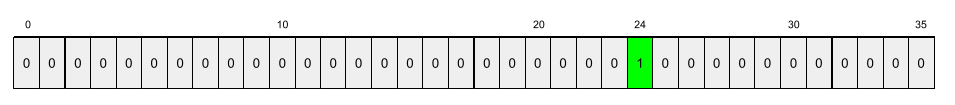
Alternatively, sparse representation would simply identify the position of the particular species. If maple is at position 24, then the sparse representation of maple would simply be:
24
Notice that the sparse representation is much more compact than the one-hot representation.
Click the icon for a slightly more complex example.
Suppose each example in your model must represent the words—but not the order of those words—in an English sentence. English consists of about 170,000 words, so English is a categorical feature with about 170,000 elements. Most English sentences use an extremely tiny fraction of those 170,000 words, so the set of words in a single example is almost certainly going to be sparse data.
Consider the following sentence:
My dog is a great dog
You could use a variant of one-hot vector to represent the words in this sentence. In this variant, multiple cells in the vector can contain a nonzero value. Furthermore, in this variant, a cell can contain an integer other than one. Although the words "my", "is", "a", and "great" appear only once in the sentence, the word "dog" appears twice. Using this variant of one-hot vectors to represent the words in this sentence yields the following 170,000-element vector:
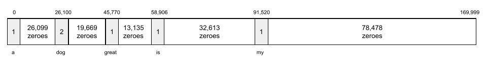
A sparse representation of the same sentence would simply be:
0: 1
26100: 2
45770: 1
58906: 1
91520: 1
See Working with categorical data in Machine Learning Crash Course for more information.
sparse vector
A vector whose values are mostly zeroes. See also sparse feature and sparsity .
sparsity
The number of elements set to zero (or null) in a vector or matrix divided by the total number of entries in that vector or matrix. For example, consider a 100-element matrix in which 98 cells contain zero. The calculation of sparsity is as follows:
Feature sparsity refers to the sparsity of a feature vector; model sparsity refers to the sparsity of the model weights.
spatial pooling
See pooling .
specificational coding
The process of writing and maintaining a file in a human language (for example, English) that describes software. You can then tell a generative AI model or another software engineer to create the software that fulfills that description.
Automatically-generated code generally requires iteration. In specificational coding, you iterate on the description file. By contrast, in conversational coding , you iterate within the prompt box. In practice, automatic code generation sometimes involves a combination of both specificational coding and conversational coding.
расколоть
In a decision tree , another name for a condition .
разветвитель
While training a decision tree , the routine (and algorithm) responsible for finding the best condition at each node .
SPMD
Abbreviation for single program / multiple data .
Отряд
Acronym for Stanford Question Answering Dataset , introduced in the paper SQuAD: 100,000+ Questions for Machine Comprehension of Text . The questions in this dataset come from people posing questions about Wikipedia articles. Some of the questions in SQuAD have answers, but other questions intentionally don't have answers. Therefore, you can use SQuAD to evaluate an LLM's ability to do both of the following:
- Answer questions that can be answered.
- Identify questions that cannot be answered.
Exact match in combination with F 1 are the most common metrics for evaluating LLMs against SQuAD.
squared hinge loss
The square of the hinge loss . Squared hinge loss penalizes outliers more harshly than regular hinge loss.
squared loss
Synonym for L 2 loss .
поэтапное обучение
A tactic of training a model in a sequence of discrete stages. The goal can be either to speed up the training process, or to achieve better model quality.
An illustration of the progressive stacking approach is shown below:
- Stage 1 contains 3 hidden layers, stage 2 contains 6 hidden layers, and stage 3 contains 12 hidden layers.
- Stage 2 begins training with the weights learned in the 3 hidden layers of Stage 1. Stage 3 begins training with the weights learned in the 6 hidden layers of Stage 2.
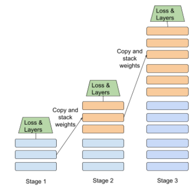
See also pipelining .
состояние
In reinforcement learning, the parameter values that describe the current configuration of the environment, which the agent uses to choose an action .
state-action value function
Synonym for Q-function .
state machine agent
An agent whose workflows are constrained by rigid rules. State machine agents generally make fewer mistakes than autonomous agents but lack the freedom to adapt to situations outside their constraints.
статический
Something done once rather than continuously. The terms static and offline are synonyms. The following are common uses of static and offline in machine learning:
- static model (or offline model ) is a model trained once and then used for a while.
- static training (or offline training ) is the process of training a static model.
- static inference (or offline inference ) is a process in which a model generates a batch of predictions at a time.
Contrast with dynamic .
static inference
Synonym for offline inference .
стационарность
A feature whose values don't change across one or more dimensions, usually time. For example, a feature whose values look about the same in 2021 and 2023 exhibits stationarity.
In the real world, very few features exhibit stationarity. Even features synonymous with stability (like sea level) change over time.
Contrast with nonstationarity .
шаг
A forward pass and backward pass of one batch .
See backpropagation for more information on the forward pass and backward pass.
step size
Synonym for learning rate .
stochastic gradient descent (SGD)
A gradient descent algorithm in which the batch size is one. In other words, SGD trains on a single example chosen uniformly at random from a training set .
See Linear regression: Hyperparameters in Machine Learning Crash Course for more information.
шаг
In a convolutional operation or pooling, the delta in each dimension of the next series of input slices. For example, the following animation demonstrates a (1,1) stride during a convolutional operation. Therefore, the next input slice starts one position to the right of the previous input slice. When the operation reaches the right edge, the next slice is all the way over to the left but one position down.
The preceding example demonstrates a two-dimensional stride. If the input matrix is three-dimensional, the stride would also be three-dimensional.
structural risk minimization (SRM)
An algorithm that balances two goals:
- The need to build the most predictive model (for example, lowest loss).
- The need to keep the model as simple as possible (for example, strong regularization).
For example, a function that minimizes loss+regularization on the training set is a structural risk minimization algorithm.
Contrast with empirical risk minimization .
sub-agent
A specialized, narrowly focused model invoked by a manager agent to handle a specific subset of a larger problem. Sub-agents typically have a narrower action space than agents.
subsampling
See pooling .
subword token
In language models , a token that is a substring of a word, which may be the entire word.
For example, a word like "itemize" might be broken up into the pieces "item" (a root word) and "ize" (a suffix), each of which is represented by its own token. Splitting uncommon words into such pieces, called subwords, allows language models to operate on the word's more common constituent parts, such as prefixes and suffixes.
Conversely, common words like "going" might not be broken up and might be represented by a single token.
краткое содержание
In TensorFlow, a value or set of values calculated at a particular step , usually used for tracking model metrics during training.
SuperGLUE
An ensemble of datasets for rating an LLM's overall ability to understand and generate text. The ensemble consists of the following datasets:
- Boolean Questions (BoolQ)
- CommitmentBank (CB)
- Choice of Plausible Alternatives (COPA)
- Multi-sentence Reading Comprehension (MultiRC)
- Reading Comprehension with Commonsense Reasoning Dataset (ReCoRD)
- Recognizing Textual Entailment (RTE)
- Words in Context (WiC)
- Winograd Schema Challenge (WSC)
For details, see SuperGLUE: A Stickier Benchmark for General-Purpose Language Understanding Systems .
supervised machine learning
Training a model from features and their corresponding labels . Supervised machine learning is analogous to learning a subject by studying a set of questions and their corresponding answers. After mastering the mapping between questions and answers, a student can then provide answers to new (never-before-seen) questions on the same topic.
Compare with unsupervised machine learning .
See Supervised Learning in the Introduction to ML course for more information.
synthetic feature
A feature not present among the input features, but assembled from one or more of them. Methods for creating synthetic features include the following:
- Bucketing a continuous feature into range bins.
- Creating a feature cross .
- Multiplying (or dividing) one feature value by other feature value(s) or by itself. For example, if
aandbare input features, then the following are examples of synthetic features:- аб
- a 2
- Applying a transcendental function to a feature value. For example, if
cis an input feature, then the following are examples of synthetic features:- sin(c)
- ln(c)
Features created by normalizing or scaling alone are not considered synthetic features.
Т
Т5
A text-to-text transfer learning model introduced by Google AI in 2020 . T5 is an encoder - decoder model, based on the Transformer architecture, trained on an extremely large dataset. It is effective at a variety of natural language processing tasks, such as generating text, translating languages, and answering questions in a conversational manner.
T5 gets its name from the five letter Ts in "Text-to-Text Transfer Transformer."
T5X
An open-source, machine learning framework designed to build and train large-scale natural language processing (NLP) models. T5 is implemented on the T5X codebase (which is built on JAX and Flax ).
tabular Q-learning
In reinforcement learning , implementing Q-learning by using a table to store the Q-functions for every combination of state and action .
цель
Synonym for label .
target network
In Deep Q-learning , a neural network that is a stable approximation of the main neural network, where the main neural network implements either a Q-function or a policy . Then, you can train the main network on the Q-values predicted by the target network. Therefore, you prevent the feedback loop that occurs when the main network trains on Q-values predicted by itself. By avoiding this feedback, training stability increases.
задача
A problem that can be solved using machine learning techniques, such as:
task decomposition
Breaking down a large goal into atomic, executable steps. Agents handle certain problems by performing task decomposition.
температура
A hyperparameter that controls the degree of randomness of a model's output. Higher temperatures result in more random output, while lower temperatures result in less random output.
Choosing the best temperature depends on the specific application and or string values.
temporal data
Data recorded at different points in time. For example, winter coat sales recorded for each day of the year would be temporal data.
Тензор
The primary data structure in TensorFlow programs. Tensors are N-dimensional (where N could be very large) data structures, most commonly scalars, vectors, or matrixes. The elements of a Tensor can hold integer, floating-point, or string values.
TensorBoard
The dashboard that displays the summaries saved during the execution of one or more TensorFlow programs.
TensorFlow
A large-scale, distributed, machine learning platform. The term also refers to the base API layer in the TensorFlow stack, which supports general computation on dataflow graphs.
Although TensorFlow is primarily used for machine learning, you may also use TensorFlow for non-ML tasks that require numerical computation using dataflow graphs.
TensorFlow Playground
A program that visualizes how different hyperparameters influence model (primarily neural network) training. Go to http://playground.tensorflow.org to experiment with TensorFlow Playground.
TensorFlow Serving
A platform to deploy trained models in production.
Tensor Processing Unit (TPU)
An application-specific integrated circuit (ASIC) that optimizes the performance of machine learning workloads. These ASICs are deployed as multiple TPU chips on a TPU device .
Tensor rank
See rank (Tensor) .
Tensor shape
The number of elements a Tensor contains in various dimensions. For example, a [5, 10] Tensor has a shape of 5 in one dimension and 10 in another.
Tensor size
The total number of scalars a Tensor contains. For example, a [5, 10] Tensor has a size of 50.
TensorStore
A library for efficiently reading and writing large multi-dimensional arrays.
termination condition
In agentic AI, the predefined criteria that tell the agent to stop iterating. For example, here are a few possible termination conditions:
- The agent successfully completed the goal.
- The agent can't use any more resources.
- A human-in-the-loop has detected a problem.
In reinforcement learning , the conditions that determine when an episode ends, such as when the agent reaches a certain state or exceeds a threshold number of state transitions. For example, in tic-tac-toe (also known as noughts and crosses), an episode terminates either when a player marks three consecutive spaces or when all spaces are marked.
тест
In a decision tree , another name for a condition .
test loss
A metric representing a model's loss against the test set . When building a model , you typically try to minimize test loss. That's because a low test loss is a stronger quality signal than a low training loss or low validation loss .
A large gap between test loss and training loss or validation loss sometimes suggests that you need to increase the regularization rate .
тестовый набор
A subset of the dataset reserved for testing a trained model .
Traditionally, you divide examples in the dataset into the following three distinct subsets:
- a training set
- a validation set
- a test set
Each example in a dataset should belong to only one of the preceding subsets. For instance, a single example shouldn't belong to both the training set and the test set.
The training set and validation set are both closely tied to training a model. Because the test set is only indirectly associated with training, test loss is a less biased, higher quality metric than training loss or validation loss .
See Datasets: Dividing the original dataset in Machine Learning Crash Course for more information.
text span
The array index span associated with a specific subsection of a text string. For example, the word good in the Python string s="Be good now" occupies the text span from 3 to 6.
tf.Example
A standard protocol buffer for describing input data for machine learning model training or inference.
tf.keras
An implementation of Keras integrated into TensorFlow .
threshold (for decision trees)
In an axis-aligned condition , the value that a feature is being compared against. For example, 75 is the threshold value in the following condition:
grade >= 75
See Exact splitter for binary classification with numerical features in the Decision Forests course for more information.
time series analysis
A subfield of machine learning and statistics that analyzes temporal data . Many types of machine learning problems require time series analysis, including classification, clustering, forecasting, and anomaly detection. For example, you could use time series analysis to forecast the future sales of winter coats by month based on historical sales data.
timestep
One "unrolled" cell within a recurrent neural network . For example, the following figure shows three timesteps (labeled with the subscripts t-1, t, and t+1):

токен
In a language model , the atomic unit that the model is training on and making predictions on. A token is typically one of the following:
- a word—for example, the phrase "dogs like cats" consists of three word tokens: "dogs", "like", and "cats".
- a character—for example, the phrase "bike fish" consists of nine character tokens. (Note that the blank space counts as one of the tokens.)
- subwords—in which a single word can be a single token or multiple tokens. A subword consists of a root word, a prefix, or a suffix. For example, a language model that uses subwords as tokens might view the word "dogs" as two tokens (the root word "dog" and the plural suffix "s"). That same language model might view the single word "taller" as two subwords (the root word "tall" and the suffix "er").
In domains outside of language models, tokens can represent other kinds of atomic units. For example, in computer vision, a token might be a subset of an image.
See Large language models in Machine Learning Crash Course for more information.
токенизатор
A system or algorithm that translates a sequence of input data into tokens .
Most modern foundation models are multimodal . A tokenizer for a multimodal system must translate each input type into the appropriate format. For example, given input data consisting of both text and graphics, the tokenizer might translate input text into subwords and input images into small patches. The tokenizer must then convert all the tokens into a single unified embedding space, which enables the model to "understand" a stream of multimodal input.
top-k accuracy
The percentage of times that a "target label" appears within the first k positions of generated lists. The lists could be personalized recommendations or a list of items ordered by softmax .
Top-k accuracy is also known as accuracy at k .
башня
A component of a deep neural network that is itself a deep neural network. In some cases, each tower reads from an independent data source, and those towers stay independent until their output is combined in a final layer. In other cases, (for example, in the encoder and decoder tower of many Transformers ), towers have cross-connections to each other.
токсичность
The degree to which content is abusive, threatening, or offensive. Many machine learning models can identify, measure, and classify toxicity. Most of these models identify toxicity along multiple parameters, such as the level of abusive language and the level of threatening language.
ТПУ
Abbreviation for Tensor Processing Unit .
TPU chip
A programmable linear algebra accelerator with on-chip high bandwidth memory that is optimized for machine learning workloads. Multiple TPU chips are deployed on a TPU device .
TPU device
A printed circuit board (PCB) with multiple TPU chips , high bandwidth network interfaces, and system cooling hardware.
TPU node
A TPU resource on Google Cloud with a specific TPU type . The TPU node connects to your VPC Network from a peer VPC network . TPU nodes are a resource defined in the Cloud TPU API .
TPU Pod
A specific configuration of TPU devices in a Google data center. All of the devices in a TPU Pod are connected to one another over a dedicated high-speed network. A TPU Pod is the largest configuration of TPU devices available for a specific TPU version.
TPU resource
A TPU entity on Google Cloud that you create, manage, or consume. For example, TPU nodes and TPU types are TPU resources.
TPU slice
A TPU slice is a fractional portion of the TPU devices in a TPU Pod . All of the devices in a TPU slice are connected to one another over a dedicated high-speed network.
TPU type
A configuration of one or more TPU devices with a specific TPU hardware version. You select a TPU type when you create a TPU node on Google Cloud. For example, a v2-8 TPU type is a single TPU v2 device with 8 cores. A v3-2048 TPU type has 256 networked TPU v3 devices and a total of 2048 cores. TPU types are a resource defined in the Cloud TPU API .
TPU worker
A process that runs on a host machine and executes machine learning programs on TPU devices .
обучение
The process of determining the ideal parameters (weights and biases) comprising a model . During training, a system reads in examples and gradually adjusts parameters. Training uses each example anywhere from a few times to billions of times.
See Supervised Learning in the Introduction to ML course for more information.
training loss
A metric representing a model's loss during a particular training iteration. For example, suppose the loss function is Mean Squared Error . Perhaps the training loss (the Mean Squared Error) for the 10th iteration is 2.2, and the training loss for the 100th iteration is 1.9.
A loss curve plots training loss versus the number of iterations. A loss curve provides the following hints about training:
- A downward slope implies that the model is improving.
- An upward slope implies that the model is getting worse.
- A flat slope implies that the model has reached convergence .
For example, the following somewhat idealized loss curve shows:
- A steep downward slope during the initial iterations, which implies rapid model improvement.
- A gradually flattening (but still downward) slope until close to the end of training, which implies continued model improvement at a somewhat slower pace then during the initial iterations.
- A flat slope towards the end of training, which suggests convergence.
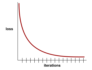
Although training loss is important, see also generalization .
training-serving skew
The difference between a model's performance during training and that same model's performance during serving .
тренировочный набор
The subset of the dataset used to train a model .
Traditionally, examples in the dataset are divided into the following three distinct subsets:
- a training set
- a validation set
- a test set
Ideally, each example in the dataset should belong to only one of the preceding subsets. For example, a single example shouldn't belong to both the training set and the validation set.
See Datasets: Dividing the original dataset in Machine Learning Crash Course for more information.
траектория
In reinforcement learning , a sequence of tuples that represent a sequence of state transitions of the agent , where each tuple corresponds to the state, action , reward , and next state for a given state transition.
transfer learning
Transferring information from one machine learning task to another. For example, in multi-task learning, a single model solves multiple tasks, such as a deep model that has different output nodes for different tasks. Transfer learning might involve transferring knowledge from the solution of a simpler task to a more complex one, or involve transferring knowledge from a task where there is more data to one where there is less data.
Most machine learning systems solve a single task. Transfer learning is a baby step towards artificial intelligence in which a single program can solve multiple tasks.
Трансформатор
A neural network architecture developed at Google that relies on self-attention mechanisms to transform a sequence of input embeddings into a sequence of output embeddings without relying on convolutions or recurrent neural networks . A Transformer can be viewed as a stack of self-attention layers.
A Transformer can include any of the following:
An encoder transforms a sequence of embeddings into a new sequence of the same length. An encoder includes N identical layers, each of which contains two sub-layers. These two sub-layers are applied at each position of the input embedding sequence, transforming each element of the sequence into a new embedding. The first encoder sub-layer aggregates information from across the input sequence. The second encoder sub-layer transforms the aggregated information into an output embedding.
A decoder transforms a sequence of input embeddings into a sequence of output embeddings, possibly with a different length. A decoder also includes N identical layers with three sub-layers, two of which are similar to the encoder sub-layers. The third decoder sub-layer takes the output of the encoder and applies the self-attention mechanism to gather information from it.
The blog post Transformer: A Novel Neural Network Architecture for Language Understanding provides a good introduction to Transformers.
See LLMs: What's a large language model? in Machine Learning Crash Course for more information.
translational invariance
In an image classification problem, an algorithm's ability to successfully classify images even when the position of objects within the image changes. For example, the algorithm can still identify a dog, whether it is in the center of the frame or at the left end of the frame.
See also size invariance and rotational invariance .
tree-of-thought prompting (ToT)
A sophisticated prompting strategy that encourages an LLM to pursue and refine the most promising intermediate solutions and to abandon the rest. Tree-of-thought prompting uses an algorithm like the following:
- Divide a complex problem into different branches (potential strategies), each comprised of multiple steps.
- Prompt the LLM to work on each branch independently.
- Ask the LLM to evaluate the quality of the solution to each branch after each step.
- Continue refining the most promising branch(es); abandon the rest.
- If a promising branch eventually fails, backtrack and try other promising steps.
триграмма
An N-gram in which N=3.
Trivia Question Answering
Datasets to evaluate an LLM's ability to answer trivia questions. Each dataset contains question-answer pairs authored by trivia enthusiasts. Different datasets are grounded by different sources, including:
- Web search (TriviaQA)
- Wikipedia (TriviaQA_wiki)
For more information see TriviaQA: A Large Scale Distantly Supervised Challenge Dataset for Reading Comprehension .
true negative (TN)
An example in which the model correctly predicts the negative class . For example, the model infers that a particular email message is not spam , and that email message really is not spam .
true positive (TP)
An example in which the model correctly predicts the positive class . For example, the model infers that a particular email message is spam, and that email message really is spam.
true positive rate (TPR)
Synonym for recall . That is:
True positive rate is the y-axis in an ROC curve .
TTL
Abbreviation for time to live .
Typologically Diverse Question Answering (TyDi QA)
A large dataset for evaluating an LLM's proficiency in answering questions. The dataset contains question and answer pairs in many languages.
For details, see TyDi QA: A Benchmark for Information-Seeking Question Answering in Typologically Diverse Languages .
У
UCR
Abbreviation for unsupported-claim rate .
Ультра
The Gemini model with the most parameters . See Gemini Ultra for details.
unawareness (to a sensitive attribute)
A situation in which sensitive attributes are present, but not included in the training data. Because sensitive attributes are often correlated with other attributes of one's data, a model trained with unawareness about a sensitive attribute could still have disparate impact with respect to that attribute, or violate other fairness constraints .
underfitting
Producing a model with poor predictive ability because the model hasn't fully captured the complexity of the training data. Many problems can cause underfitting, including:
- Training on the wrong set of features .
- Training for too few epochs or at too low a learning rate .
- Training with too high a regularization rate .
- Providing too few hidden layers in a deep neural network.
See Overfitting in Machine Learning Crash Course for more information.
undersampling
Removing examples from the majority class in a class-imbalanced dataset in order to create a more balanced training set .
For example, consider a dataset in which the ratio of the majority class to the minority class is 20:1. To overcome this class imbalance, you could create a training set consisting of all of the minority class examples but only a tenth of the majority class examples, which would create a training-set class ratio of 2:1. Thanks to undersampling, this more balanced training set might produce a better model. Alternatively, this more balanced training set might contain insufficient examples to train an effective model.
Contrast with oversampling .
однонаправленный
A system that only evaluates the text that precedes a target section of text. In contrast, a bidirectional system evaluates both the text that precedes and follows a target section of text. See bidirectional for more details.
unidirectional language model
A language model that bases its probabilities only on the tokens appearing before , not after , the target token(s). Contrast with bidirectional language model .
unlabeled example
An example that contains features but no label . For example, the following table shows three unlabeled examples from a house valuation model, each with three features but no house value:
| Количество спален | Количество ванных комнат | House age |
|---|---|---|
| 3 | 2 | 15 |
| 2 | 1 | 72 |
| 4 | 2 | 34 |
In supervised machine learning , models train on labeled examples and make predictions on unlabeled examples .
In semi-supervised and unsupervised learning, unlabeled examples are used during training.
Contrast unlabeled example with labeled example .
unsupervised machine learning
Training a model to find patterns in a dataset, typically an unlabeled dataset.
The most common use of unsupervised machine learning is to cluster data into groups of similar examples. For example, an unsupervised machine learning algorithm can cluster songs based on various properties of the music. The resulting clusters can become an input to other machine learning algorithms (for example, to a music recommendation service). Clustering can help when useful labels are scarce or absent. For example, in domains such as anti-abuse and fraud, clusters can help humans better understand the data.
Contrast with supervised machine learning .
See What is Machine Learning? in the Introduction to ML course for more information.
unsupported-claim rate (UCR)
The percentage of claims in a response that aren't grounded . For example, if an LLM's response makes 10 claims but only 1 is grounded, the UCR is 90%.
A high UCR implies that an LLM is hallucinating too frequently.
See also citation precision and citation recall .
uplift modeling
A modeling technique, commonly used in marketing, that models the "causal effect" (also known as the "incremental impact") of a "treatment" on an "individual." Here are two examples:
- Doctors might use uplift modeling to predict the mortality decrease (causal effect) of a medical procedure (treatment) depending on the age and medical history of a patient (individual).
- Marketers might use uplift modeling to predict the increase in probability of a purchase (causal effect) due to an advertisement (treatment) on a person (individual).
Uplift modeling differs from classification or regression in that some labels (for example, half of the labels in binary treatments) are always missing in uplift modeling. For example, a patient can either receive or not receive a treatment; therefore, we can only observe whether the patient is going to heal or not heal in only one of these two situations (but never both). The main advantage of an uplift model is that it can generate predictions for the unobserved situation (the counterfactual) and use it to compute the causal effect.
upweighting
Applying a weight to the downsampled class equal to the factor by which you downsampled.
user matrix
In recommendation systems , an embedding vector generated by matrix factorization that holds latent signals about user preferences. Each row of the user matrix holds information about the relative strength of various latent signals for a single user. For example, consider a movie recommendation system. In this system, the latent signals in the user matrix might represent each user's interest in particular genres, or might be harder-to-interpret signals that involve complex interactions across multiple factors.
The user matrix has a column for each latent feature and a row for each user. That is, the user matrix has the same number of rows as the target matrix that is being factorized. For example, given a movie recommendation system for 1,000,000 users, the user matrix will have 1,000,000 rows.
В
валидация
The initial evaluation of a model's quality. Validation checks the quality of a model's predictions against the validation set .
Because the validation set differs from the training set , validation helps guard against overfitting .
You might think of evaluating the model against the validation set as the first round of testing and evaluating the model against the test set as the second round of testing.
validation loss
A metric representing a model's loss on the validation set during a particular iteration of training.
See also generalization curve .
набор валидации
The subset of the dataset that performs initial evaluation against a trained model . Typically, you evaluate the trained model against the validation set several times before evaluating the model against the test set .
Traditionally, you divide the examples in the dataset into the following three distinct subsets:
- a training set
- a validation set
- a test set
Ideally, each example in the dataset should belong to only one of the preceding subsets. For example, a single example shouldn't belong to both the training set and the validation set.
See Datasets: Dividing the original dataset in Machine Learning Crash Course for more information.
value imputation
The process of replacing a missing value with an acceptable substitute. When a value is missing, you can either discard the entire example or you can use value imputation to salvage the example.
For example, consider a dataset containing a temperature feature that is supposed to be recorded every hour. However, the temperature reading was unavailable for a particular hour. Here is a section of the dataset:
| Отметка времени | Температура |
|---|---|
| 1680561000 | 10 |
| 1680564600 | 12 |
| 1680568200 | отсутствующий |
| 1680571800 | 20 |
| 1680575400 | 21 |
| 1680579000 | 21 |
A system could either delete the missing example or impute the missing temperature as 12, 16, 18, or 20, depending on the imputation algorithm.
vanishing gradient problem
The tendency for the gradients of early hidden layers of some deep neural networks to become surprisingly flat (low). Increasingly lower gradients result in increasingly smaller changes to the weights on nodes in a deep neural network, leading to little or no learning. Models suffering from the vanishing gradient problem become difficult or impossible to train. Long Short-Term Memory cells address this issue.
Compare to exploding gradient problem .
variable importances
A set of scores that indicates the relative importance of each feature to the model.
For example, consider a decision tree that estimates house prices. Suppose this decision tree uses three features: size, age, and style. If a set of variable importances for the three features are calculated to be {size=5.8, age=2.5, style=4.7}, then size is more important to the decision tree than age or style.
Different variable importance metrics exist, which can inform ML experts about different aspects of models.
variational autoencoder (VAE)
A type of autoencoder that leverages the discrepancy between inputs and outputs to generate modified versions of the inputs. Variational autoencoders are useful for generative AI .
VAEs are based on variational inference: a technique for estimating the parameters of a probability model.
вектор
Very overloaded term whose meaning varies across different mathematical and scientific fields. Within machine learning, a vector has two properties:
- Data type: Vectors in machine learning usually hold floating-point numbers.
- Number of elements: This is the vector's length or its dimension .
For example, consider a feature vector that holds eight floating-point numbers. This feature vector has a length or dimension of eight. Note that machine learning vectors often have a huge number of dimensions.
You can represent many different kinds of information as a vector. For example:
- Any position on the surface of Earth can be represented as a 2-dimensional vector, where one dimension is the latitude and the other is the longitude.
- The current prices of each of 500 stocks can be represented as a 500-dimensional vector.
- A probability distribution over a finite number of classes can be represented as a vector. For example, a multiclass classification system that predicts one of three output colors (red, green, or yellow) could output the vector
(0.3, 0.2, 0.5)to meanP[red]=0.3, P[green]=0.2, P[yellow]=0.5.
Vectors can be concatenated; therefore, a variety of different media can be represented as a single vector. Some models operate directly on the concatenation of many one-hot encodings .
Specialized processors such as TPUs are optimized to perform mathematical operations on vectors.
A vector is a tensor of rank 1.
Вершина
Google Cloud's platform for AI and machine learning. Vertex provides tools and infrastructure for building, deploying, and managing AI applications, including access to Gemini models.кодирование вибрации
Prompting a generative AI model to create software. That is, your prompts describe the software's purpose and features, which a generative AI model translates into source code. The generated code doesn't always match your intentions, so vibe coding usually requires iteration.
Andrej Karpathy coined the term vibe coding in this X post . In the X post, Karpathy describes it as "a new kind of coding...where you fully give in to the vibes..." So, the term originally implied an intentionally loose approach to creating software in which you might not even examine the generated code. However, the term has rapidly evolved in many circles to now mean any form of AI-generated coding.
For a more detailed description of vibe coding, seeWhat is vibe coding? .
In addition, compare and contrast vibe coding with:
В
Wasserstein loss
One of the loss functions commonly used in generative adversarial networks , based on the earth mover's distance between the distribution of generated data and real data.
масса
A value that a model multiplies by another value. Training is the process of determining a model's ideal weights; inference is the process of using those learned weights to make predictions.
See Linear regression in Machine Learning Crash Course for more information.
Weighted Alternating Least Squares (WALS)
An algorithm for minimizing the objective function during matrix factorization in recommendation systems , which allows a downweighting of the missing examples. WALS minimizes the weighted squared error between the original matrix and the reconstruction by alternating between fixing the row factorization and column factorization. Each of these optimizations can be solved by least squares convex optimization . For details, see the Recommendation Systems course .
weighted sum
The sum of all the relevant input values multiplied by their corresponding weights. For example, suppose the relevant inputs consist of the following:
| входное значение | input weight |
| 2 | -1.3 |
| -1 | 0,6 |
| 3 | 0,4 |
The weighted sum is therefore:
weighted sum = (2)(-1.3) + (-1)(0.6) + (3)(0.4) = -2.0
A weighted sum is the input argument to an activation function .
WiC
Abbreviation for Words in Context .
wide model
A linear model that typically has many sparse input features . We refer to it as "wide" since such a model is a special type of neural network with a large number of inputs that connect directly to the output node. Wide models are often easier to debug and inspect than deep models . Although wide models cannot express nonlinearities through hidden layers , wide models can use transformations such as feature crossing and bucketization to model nonlinearities in different ways.
Contrast with deep model .
ширина
The number of neurons in a particular layer of a neural network .
WikiLingua (wiki_lingua)
A dataset for evaluating an LLM's ability to summarize short articles. WikiHow , an encyclopedia of articles explaining how to do various tasks, is the human-authored source for both the articles and the summaries. Each entry in the dataset consists of:
- An article, which is created by appending each step of the prose (paragraph) version of the numbered list, minus the opening sentence of each step.
- A summary of that article, consisting of the opening sentence of each step in the numbered list.
For details, see WikiLingua: A New Benchmark Dataset for Cross-Lingual Abstractive Summarization .
Winograd Schema Challenge (WSC)
A format (or dataset conforming to that format) for evaluating an LLM's ability to determine the noun phrase that a pronoun refers to.
Each entry in a Winograd Schema Challenge consists of:
- A short passage, which contains a target pronoun
- A target pronoun
- Candidate noun phrases, followed by the correct answer (a Boolean). If the target pronoun refers to this candidate, the answer is True. If the target pronoun does not refer to this candidate, the answer is False.
Например:
- Passage : Mark told Pete many lies about himself, which Pete included in his book. He should have been more truthful.
- Target pronoun : He
- Candidate noun phrases :
- Mark: True, because the target pronoun refers to Mark
- Pete: False, because the target pronoun doesn't refer to Peter
The Winograd Schema Challenge is a component of the SuperGLUE ensemble.
wisdom of the crowd
The idea that averaging the opinions or estimates of a large group of people ("the crowd") often produces surprisingly good results. For example, consider a game in which people guess the number of jelly beans packed into a large jar. Although most individual guesses will be inaccurate, the average of all the guesses has been empirically shown to be surprisingly close to the actual number of jelly beans in the jar.
Ensembles are a software analog of wisdom of the crowd. Even if individual models make wildly inaccurate predictions, averaging the predictions of many models often generates surprisingly good predictions. For example, although an individual decision tree might make poor predictions, a decision forest often makes very good predictions.
WMT
Strangely, an abbreviation for Conference on Machine Translation . (The abbreviation is W MT because the original name was Workshop on Machine Translation.) The conference focuses on developments in machine translation systems.
word embedding
Representing each word in a word set within an embedding vector ; that is, representing each word as a vector of floating-point values between 0.0 and 1.0. Words with similar meanings have more-similar representations than words with different meanings. For example, carrots , celery , and cucumbers would all have relatively similar representations, which would be very different from the representations of airplane , sunglasses , and toothpaste .
Words in Context (WiC)
A dataset for evaluating how well an LLM uses context to understand words that have multiple meanings. Each entry in the dataset contains:
- Two sentences, each containing the target word
- The target word
- The correct answer (a Boolean), where:
- True means the target word has the same meaning in the two sentences
- False means the target word has a different meaning in the two sentences
Например:
- Two sentences:
- There's a lot of trash on the bed of the river.
- I keep a glass of water next to my bed when I sleep.
- The target word: bed
- Correct answer : False, because the target word has a different meaning in the two sentences.
For details, see WiC: the Word-in-Context Dataset for Evaluating Context-Sensitive Meaning Representations .
Words in Context is a component of the SuperGLUE ensemble.
WSC
Abbreviation for Winograd Schema Challenge .
X
XLA (Accelerated Linear Algebra)
An open-source machine learning compiler for GPUs, CPUs, and ML accelerators.
The XLA compiler takes models from popular ML frameworks such as PyTorch , TensorFlow , and JAX , and optimizes them for high-performance execution across different hardware platforms including GPUs, CPUs, and ML accelerators .
XL-Sum (xlsum)
A dataset for evaluating an LLM's proficiency in summarizing text. XL-Sum provides entries in many languages. Each entry in the dataset contains:
- An article, taken from the British Broadcasting Company (BBC).
- A summary of the article, written by the article's author. Note that that summary can contain words or phrases not present in the article.
For details, see XL-Sum: Large-Scale Multilingual Abstractive Summarization for 44 Languages .
xsum
Abbreviation for Extreme Summarization .
З
zero-shot learning
A type of machine learning training where the model infers a prediction for a task that it was not specifically already trained on. In other words, the model is given zero task-specific training examples but asked to do inference for that task.
zero-shot prompting
A prompt that does not provide an example of how you want the large language model to respond. For example:
| Parts of one prompt | Примечания |
|---|---|
| What is the official currency of the specified country? | The question you want the LLM to answer. |
| Индия: | The actual query. |
The large language model might respond with any of the following:
- Рупия
- мРНК
- ₹
- индийская рупия
- The rupee
- The Indian rupee
All of the answers are correct, though you might prefer a particular format.
Compare and contrast zero-shot prompting with the following terms:
Z-score normalization
A scaling technique that replaces a raw feature value with a floating-point value representing the number of standard deviations from that feature's mean. For example, consider a feature whose mean is 800 and whose standard deviation is 100. The following table shows how Z-score normalization would map the raw value to its Z-score:
| Raw value | Z-score |
|---|---|
| 800 | 0 |
| 950 | +1.5 |
| 575 | -2.25 |
The machine learning model then trains on the Z-scores for that feature instead of on the raw values.
See Numerical data: Normalization in Machine Learning Crash Course for more information.
,В этом глоссарии даны определения терминов, связанных с искусственным интеллектом.
А
абляция
Метод оценки важности признака или компонента путем его временного удаления из модели . Затем модель переобучается без этого признака или компонента, и если переобученная модель показывает значительно худшие результаты, то удаленный признак или компонент, вероятно, был важен.
Например, предположим, вы обучили модель классификации на 10 признаках и достигли точности 88% на тестовом наборе . Чтобы проверить важность первого признака, вы можете переобучить модель, используя только девять других признаков. Если переобученная модель показывает значительно худшие результаты (например, точность 55%), то, вероятно, удаленный признак был важен. И наоборот, если переобученная модель показывает такие же хорошие результаты, то, вероятно, этот признак был не так уж важен.
Абляция также может помочь определить значимость следующих факторов:
- Более крупные компоненты, такие как целая подсистема более крупной системы машинного обучения.
- Процессы или методы, например, этап предварительной обработки данных.
В обоих случаях вы сможете наблюдать, как изменяется (или не изменяется) производительность системы после удаления компонента.
A/B-тестирование
Статистический способ сравнения двух (или более) методов — A и B. Как правило, A — это уже существующий метод, а B — новый. A/B-тестирование позволяет не только определить, какой метод работает лучше, но и выяснить, является ли разница статистически значимой.
A/B-тестирование обычно сравнивает один показатель по двум методам; например, как точность модели соотносится с точностью двух методов? Однако A/B-тестирование может также сравнивать любое конечное число показателей.
чип-ускоритель
Категория специализированных аппаратных компонентов, предназначенных для выполнения ключевых вычислений, необходимых для алгоритмов глубокого обучения.
Ускорительные чипы (или просто ускорители ) могут значительно повысить скорость и эффективность задач обучения и вывода по сравнению с центральным процессором общего назначения. Они идеально подходят для обучения нейронных сетей и аналогичных ресурсоемких вычислительных задач.
Примерами микросхем-ускорителей являются:
- Тензорные процессоры Google ( TPU ) со специализированным оборудованием для глубокого обучения.
- Графические процессоры NVIDIA, хотя и были изначально разработаны для обработки графики, позволяют использовать параллельную обработку, что может значительно повысить скорость обработки.
точность
Количество правильных классификационных прогнозов, деленное на общее количество прогнозов. То есть:
Например, модель, сделавшая 40 правильных и 10 неправильных прогнозов, будет иметь точность:
Бинарная классификация предоставляет конкретные названия для различных категорий правильных и неправильных прогнозов . Таким образом, формула точности для бинарной классификации выглядит следующим образом:
где:
- TP — это количество истинно положительных результатов (правильных прогнозов).
- TN — это количество истинно отрицательных результатов (правильных предсказаний).
- FP — это количество ложноположительных результатов (неверных прогнозов).
- FN — это количество ложноотрицательных результатов (неверных прогнозов).
Сравните и сопоставьте точность с прецизией и полнотой .
Дополнительную информацию см. в разделе «Классификация: точность, полнота, прецизионность и связанные с ними показатели» в кратком курсе по машинному обучению.
действовать
Этап в цикле работы агента, на котором агент выполняет действие, выбранное на этапе обоснования . Например, на этапе выполнения действия может быть отправлен API-запрос.
действие
В обучении с подкреплением механизм, посредством которого агент переходит между состояниями окружающей среды , заключается в выборе действия с использованием стратегии .
пространство действий
Пространство действий — это набор ресурсов, которые агент может использовать для выполнения задачи. В него могут входить инструменты и API, которые агент может вызывать, а также его права доступа. В целом, пространство действий должно быть достаточно большим, чтобы агент мог выполнить задачу. Если пространство действий слишком мало, у агента может не хватать ресурсов для выполнения задачи. Если же пространство действий слишком велико, агент, как правило, становится более склонен к ошибкам.
функция активации
Функция, позволяющая нейронным сетям изучать нелинейные (сложные) взаимосвязи между признаками и меткой.
К популярным функциям активации относятся:
Графики функций активации никогда не представляют собой одну прямую линию. Например, график функции активации ReLU состоит из двух прямых линий:
График сигмоидной функции активации выглядит следующим образом:
Нажмите на значок, чтобы увидеть пример.
В нейронной сети функции активации обрабатывают взвешенную сумму всех входных сигналов нейрона . Для вычисления взвешенной суммы нейрон суммирует произведения соответствующих значений и весов. Например, предположим, что соответствующие входные сигналы для нейрона состоят из следующего:
| входное значение | входной вес |
| 2 | -1.3 |
| -1 | 0,6 |
| 3 | 0,4 |
weighted sum = (2)(-1.3) + (-1)(0.6) + (3)(0.4) = -2.0
Дополнительную информацию можно найти в разделе «Нейронные сети: функции активации» в кратком курсе по машинному обучению.
активное обучение
Активное обучение — это подход к обучению , при котором алгоритм выбирает часть данных, на которых он обучается. Оно особенно ценно, когда размеченные примеры редки или их получение обходится дорого. Вместо того чтобы слепо искать разнообразный набор размеченных примеров, алгоритм активного обучения избирательно ищет именно тот набор примеров, который ему необходим для обучения.
АдаГрад
Сложный алгоритм градиентного спуска, который масштабирует градиенты каждого параметра , фактически задавая каждому параметру независимую скорость обучения . Подробное объяснение см. в разделе «Адаптивные субградиентные методы для онлайн-обучения и стохастической оптимизации» .
приспособление
Синоним к слову «настройка» или «тонкая настройка» .
агент
Программное обеспечение, способное анализировать вводимые пользователем данные для планирования и выполнения действий от его имени.
В обучении с подкреплением агент — это сущность, которая использует стратегию для максимизации ожидаемой отдачи от перехода между состояниями окружающей среды .
агентный
Прилагательная форма слова «агент» . «Агентный» относится к качествам, которыми обладают агенты (например, автономия).
агентный цикл
Цикл, который агент проходит до тех пор, пока не будет выполнено условие завершения . Цикл обычно состоит из следующих четырех этапов:
агентский рабочий процесс
Динамический процесс, в котором агент автономно планирует и выполняет действия для достижения цели. Этот процесс может включать рассуждения, использование внешних инструментов и самокоррекцию плана.
оркестрация агентов
Централизованное управление и маршрутизация задач между несколькими суб-агентами или вызовами LLM. Управление работой агентов разбивает сложные задачи на более мелкие подзадачи и назначает их наиболее компетентным суб-агентам.
агломеративная кластеризация
См. иерархическую кластеризацию .
AI slop
Результат работы генеративной системы искусственного интеллекта , которая отдает предпочтение количеству, а не качеству. Например, веб-страница, созданная с помощью ИИ, заполнена дешевым, сгенерированным ИИ, низкокачественным контентом.
обнаружение аномалий
Процесс выявления выбросов . Например, если среднее значение для определенного параметра равно 100 со стандартным отклонением 10, то система обнаружения аномалий должна пометить значение 200 как подозрительное.
АР
Сокращение от «дополненная реальность» .
площадь под кривой PR
См. PR AUC (площадь под кривой PR) .
площадь под кривой ROC
См. AUC (площадь под ROC-кривой) .
искусственный общий интеллект
Нечеловеческий механизм, демонстрирующий широкий спектр способностей к решению проблем, креативность и адаптивность. Например, программа, демонстрирующая искусственный общий интеллект, могла бы переводить текст, сочинять симфонии и преуспевать в играх, которые еще не изобретены.
искусственный интеллект
Нечеловеческая программа или модель , способная решать сложные задачи. Например, программа или модель, переводящая текст, или программа или модель, определяющая заболевания по рентгеновским снимкам, — обе демонстрируют искусственный интеллект.
Формально машинное обучение является подразделом искусственного интеллекта. Однако в последние годы некоторые организации стали использовать термины «искусственный интеллект» и «машинное обучение» как взаимозаменяемые.
внимание
Механизм внимания, используемый в нейронной сети , который указывает на важность конкретного слова или части слова. Внимание сжимает объем информации, необходимой модели для прогнозирования следующего токена/слова. Типичный механизм внимания может представлять собой взвешенную сумму по набору входных данных, где вес для каждого входного значения вычисляется другой частью нейронной сети.
Обратите также внимание на самовнимание и многоголовочное самовнимание , которые являются строительными блоками трансформеров .
Дополнительную информацию о механизме самовнимания см. в статье «LLMs: What's a large language model?» в сборнике «Machine Learning Crash Course».
атрибут
Синоним к слову "функция" .
В контексте машинного обучения под атрибутами часто подразумеваются характеристики, относящиеся к отдельным лицам.
выборка атрибутов
Тактика обучения дерева решений, при которой каждое дерево решений рассматривает только случайное подмножество возможных признаков при изучении условия . Как правило, для каждого узла выбирается разное подмножество признаков. В отличие от этого, при обучении дерева решений без выборки атрибутов для каждого узла рассматриваются все возможные признаки.
AUC (Площадь под ROC-кривой)
Число от 0,0 до 1,0, представляющее способность модели бинарной классификации разделять положительные и отрицательные классы . Чем ближе AUC к 1,0, тем лучше модель способна разделять классы.
Например, на следующем рисунке показана модель классификации , которая идеально разделяет положительные классы (зеленые овалы) от отрицательных классов (фиолетовые прямоугольники). Эта нереалистично идеальная модель имеет показатель AUC, равный 1,0:
Напротив, на следующем рисунке показаны результаты для модели классификации , которая генерировала случайные результаты. Для этой модели показатель AUC равен 0,5:
Да, у предыдущей модели показатель AUC равен 0,5, а не 0,0.
Большинство моделей находятся где-то между этими двумя крайностями. Например, следующая модель несколько разделяет положительные и отрицательные значения, и поэтому имеет AUC где-то между 0,5 и 1,0:
AUC игнорирует любые значения, которые вы задаете для порога классификации . Вместо этого AUC учитывает все возможные пороги классификации.
Нажмите на значок, чтобы узнать о взаимосвязи между AUC и ROC-кривыми.
AUC представляет собой площадь под ROC-кривой . Например, ROC-кривая для модели, которая идеально разделяет положительные и отрицательные результаты, выглядит следующим образом:
AUC — это площадь серой области на предыдущем рисунке. В этом необычном случае площадь — это просто длина серой области (1,0), умноженная на ширину серой области (1,0). Таким образом, произведение 1,0 и 1,0 дает AUC, равное ровно 1,0, что является максимально возможным значением AUC.
Напротив, ROC-кривая для модели классификации , которая вообще не может разделять классы, выглядит следующим образом. Площадь этой серой области составляет 0,5.
Типичная ROC-кривая выглядит примерно так:
Вычисление площади под этой кривой вручную было бы трудоемким процессом, поэтому большинство значений AUC обычно рассчитываются программами.
Дополнительную информацию см. в разделе «Классификация: ROC и AUC в экспресс-курсе по машинному обучению».
дополненная реальность
Технология, которая накладывает сгенерированное компьютером изображение на реальное изображение, видимое пользователем, создавая таким образом составное изображение.
автокодировщик
Система, которая учится извлекать наиболее важную информацию из входных данных. Автокодировщики представляют собой комбинацию кодировщика и декодера . Автокодировщики используют следующий двухэтапный процесс:
- Кодировщик преобразует входные данные в (как правило) формат с потерями, имеющий промежуточную размерность.
- Декодер создает версию исходного входного сигнала с потерями, отображая формат меньшей размерности на исходный формат входного сигнала большей размерности.
Автокодировщики обучаются сквозным методом, при котором декодер пытается максимально точно восстановить исходный входной сигнал из промежуточного формата кодировщика. Поскольку промежуточный формат меньше (менее размерен), чем исходный формат, автокодировщик вынужден изучать, какая информация во входных данных является существенной, и выходные данные не будут идеально идентичны входным.
Например:
- Если входные данные представляют собой графическое изображение, то неточная копия будет похожа на исходное изображение, но несколько изменена. Возможно, неточная копия удаляет шум из исходного изображения или заполняет некоторые недостающие пиксели.
- Если входные данные представляют собой текст, автокодировщик сгенерирует новый текст, который будет имитировать (но не идентичен) исходному тексту.
См. также вариационные автокодировщики .
автоматическая оценка
Использование программного обеспечения для оценки качества результатов работы модели.
Когда выходные данные модели относительно просты, скрипт или программа могут сравнить выходные данные модели с эталонным ответом . Этот тип автоматической оценки иногда называют программной оценкой . Для программной оценки часто полезны такие метрики, как ROUGE или BLEU .
Когда результаты работы модели сложны или не имеют единственно правильного ответа , иногда автоматическую оценку выполняет отдельная программа машинного обучения, называемая авторизатором .
Сравните с человеческой оценкой .
предвзятость автоматизации
Когда человек, принимающий решения, отдает предпочтение рекомендациям автоматизированной системы принятия решений перед информацией, полученной без автоматизации, даже если автоматизированная система принятия решений допускает ошибки.
Дополнительную информацию см. в разделе «Справедливость: виды предвзятости в экспресс-курсе по машинному обучению».
AutoML
Любой автоматизированный процесс построения моделей машинного обучения . AutoML может автоматически выполнять такие задачи, как:
- Найдите наиболее подходящую модель.
- Настройте гиперпараметры .
- Подготовка данных (включая выполнение инженерии признаков ).
- Разверните полученную модель.
AutoML полезен для специалистов по обработке данных, поскольку позволяет сэкономить время и усилия при разработке конвейеров машинного обучения и повысить точность прогнозирования. Он также полезен для неспециалистов, делая сложные задачи машинного обучения более доступными для них.
Дополнительную информацию см. в разделе «Автоматизированное машинное обучение (AutoML)» в «Кратком курсе по машинному обучению».
автономный агент
Агент, который работает над достижением сложной цели, планируя, действуя и адаптируясь без постоянного вмешательства человека.
авторская оценка
Гибридный механизм оценки качества результатов работы генеративной модели ИИ , сочетающий в себе оценку человеком и автоматическую оценку . Авторефер — это модель машинного обучения, обученная на данных, созданных в результате оценки человеком . В идеале авторефер учится имитировать действия человека-оценщика.В продаже имеются готовые автоматизированные системы оценки, но лучшие из них специально оптимизированы для решения конкретной задачи.
авторегрессионная модель
Модель , которая делает вывод на основе собственных предыдущих прогнозов. Например, авторегрессивные языковые модели прогнозируют следующий токен на основе ранее предсказанных токенов. Все большие языковые модели на основе Transformer являются авторегрессивными.
В отличие от них, модели обработки изображений на основе GAN обычно не являются авторегрессивными, поскольку они генерируют изображение за один прямой проход, а не итеративно пошагово. Однако некоторые модели генерации изображений являются авторегрессивными, поскольку они генерируют изображение пошагово.
вспомогательные потери
Функция потерь — используемая совместно с основной функцией потерь модели нейронной сети — помогает ускорить обучение на ранних итерациях, когда веса инициализируются случайным образом.
Вспомогательные функции потерь переносят эффективные градиенты на более ранние слои . Это способствует сходимости во время обучения , борясь с проблемой затухания градиента .
средняя точность при k
Метрика, суммирующая производительность модели при обработке одного запроса, генерирующего ранжированные результаты, например, нумерованный список рекомендаций книг. Средняя точность в точке k — это, собственно, среднее значение точности в точке k для каждого релевантного результата. Формула для расчета средней точности в точке k выглядит следующим образом:
\[{\text{average precision at k}} = \frac{1}{n} \sum_{i=1}^n {\text{precision at k for each relevant item} } \]
где:
- \(n\) — это количество релевантных элементов в списке.
Сравните с результатами запоминания в точке k .
условие выравнивания по осям
В дереве решений условие , включающее только один признак . Например, если признаком является area , то следующее условие соответствует оси распределения:
area > 200
Сравните с косым расположением .
Б
обратное распространение
Алгоритм, реализующий градиентный спуск в нейронных сетях .
Обучение нейронной сети включает в себя множество итераций следующего двухэтапного цикла:
- В процессе прямого прохода система обрабатывает пакет примеров для получения прогнозов. Система сравнивает каждый прогноз с каждым значением метки . Разница между прогнозом и значением метки представляет собой ошибку для данного примера. Система суммирует ошибки для всех примеров, чтобы вычислить общую ошибку для текущего пакета.
- В процессе обратного распространения ошибки система уменьшает потери, корректируя веса всех нейронов во всех скрытых слоях .
Нейронные сети часто содержат множество нейронов в различных скрытых слоях. Каждый из этих нейронов вносит свой вклад в общую функцию потерь. Обратное распространение ошибки определяет, следует ли увеличивать или уменьшать веса, применяемые к конкретным нейронам.
Скорость обучения — это множитель, который регулирует степень увеличения или уменьшения каждого веса при каждом обратном проходе. Высокая скорость обучения будет увеличивать или уменьшать каждый вес сильнее, чем низкая скорость обучения.
В терминах математического анализа, обратное распространение ошибки реализует правило цепочки из математического анализа. То есть, обратное распространение ошибки вычисляет частную производную ошибки по каждому параметру.
Несколько лет назад специалистам по машинному обучению приходилось писать код для реализации обратного распространения ошибки. Современные API для машинного обучения, такие как Keras, теперь реализуют обратное распространение ошибки автоматически. Уф!
Для получения более подробной информации см. раздел «Нейронные сети в кратком курсе по машинному обучению».
упаковка
Метод обучения ансамбля , в котором каждая составляющая модель обучается на случайном подмножестве обучающих примеров, выбранных с замещением . Например, случайный лес — это набор деревьев решений, обученных с помощью метода бэггинга.
Термин bagging является сокращением от bootstrap aggregate .
Дополнительную информацию см. в разделе «Случайные леса» курса «Лесорешения».
мешок слов
Представление слов во фразе или отрывке текста независимо от порядка их следования. Например, «мешок слов» идентично представляет следующие три фразы:
- собака прыгает
- прыгает на собаку
- собака перепрыгивает
Каждое слово сопоставляется с индексом в разреженном векторе , где вектор содержит индекс для каждого слова в словаре. Например, фраза «собака прыгает» сопоставляется с вектором признаков, имеющим ненулевые значения в трех индексах, соответствующих словам «собака» , «собака» и «прыгает» . Ненулевое значение может быть любым из следующих:
- Цифра 1 обозначает наличие слова.
- Подсчет количества вхождений слова в набор. Например, если фраза "were the maroon dog is a dog with maroon fur" (бордовая собака — собака с бордовой шерстью) , то слова "maroon" и "dog" будут представлены как 2, а остальные слова — как 1.
- Какое-либо другое значение, например, логарифм количества появлений слова в мешке.
исходный уровень
Модель, используемая в качестве эталона для сравнения эффективности другой модели (как правило, более сложной). Например, модель логистической регрессии может служить хорошей базовой моделью для глубокой модели .
Для решения конкретной задачи базовый уровень помогает разработчикам моделей количественно оценить минимальную ожидаемую производительность, которую должна достичь новая модель, чтобы быть полезной.
базовая модель
Предварительно обученная модель , которая может служить отправной точкой для тонкой настройки с целью решения конкретных задач или приложений.
См. также предварительно обученную модель и базовую модель .
партия
Набор примеров, используемых в одной итерации обучения. Размер пакета определяет количество примеров в пакете.
См. раздел «Эпоха» для объяснения того, как пакет данных соотносится с эпохой.
Для получения более подробной информации см. статью «Линейная регрессия: гиперпараметры в машинном обучении».
пакетный вывод
Процесс вывода прогнозов на основе множества немаркированных примеров, разделенных на более мелкие подмножества («пакеты»).
Пакетный вывод может использовать преимущества возможностей распараллеливания, предоставляемых чипами ускорителей . То есть, несколько ускорителей могут одновременно делать прогнозы на разных пакетах немаркированных примеров, что значительно увеличивает количество выводов в секунду.
Дополнительную информацию можно найти в разделе «Системы машинного обучения в производственной среде: статический и динамический вывод» в «Кратком курсе по машинному обучению».
пакетная нормализация
Нормализация входных или выходных данных функций активации в скрытом слое . Пакетная нормализация может обеспечить следующие преимущества:
- Повысьте стабильность нейронных сетей , защитив их от выбросов в весовых коэффициентах.
- Необходимо обеспечить более высокую скорость обучения , что может ускорить тренировку.
- Уменьшите переобучение .
размер партии
Количество примеров в пакете . Например, если размер пакета равен 100, то модель обрабатывает 100 примеров за итерацию .
Ниже представлены популярные стратегии определения размера партии:
- Стохастический градиентный спуск (SGD) , в котором размер пакета равен 1.
- Полный пакет (Full batch) — это стратегия, в которой размер пакета равен количеству примеров во всем обучающем наборе данных . Например, если обучающий набор содержит миллион примеров, то размер пакета будет равен миллиону примеров. Стратегия полного пакета обычно неэффективна.
- Мини-партии, размер партии которых обычно составляет от 10 до 1000 единиц. Мини-партии, как правило, являются наиболее эффективной стратегией.
Дополнительную информацию см. ниже:
- Системы машинного обучения для производственных целей: статический и динамический вывод в кратком курсе по машинному обучению.
- Руководство по настройке глубокого обучения .
Байесовская нейронная сеть
Вероятностная нейронная сеть , учитывающая неопределенность весов и выходных данных. Стандартная модель регрессии на основе нейронной сети обычно предсказывает скалярное значение; например, стандартная модель предсказывает цену дома в 853 000. В отличие от этого, байесовская нейронная сеть предсказывает распределение значений; например, байесовская модель предсказывает цену дома в 853 000 со стандартным отклонением 67 200.
Байесовская нейронная сеть использует теорему Байеса для вычисления неопределенностей в весах и прогнозах. Байесовская нейронная сеть может быть полезна, когда важно количественно оценить неопределенность, например, в моделях, связанных с фармацевтикой. Байесовские нейронные сети также могут помочь предотвратить переобучение .
Байесовская оптимизация
Метод вероятностной регрессионной модели для оптимизации ресурсоемких целевых функций путем оптимизации аппроксимирующей функции, которая количественно оценивает неопределенность с помощью байесовского обучения. Поскольку байесовская оптимизация сама по себе очень затратна, она обычно используется для оптимизации сложных задач с небольшим количеством параметров, таких как выбор гиперпараметров .
Уравнение Беллмана
В обучении с подкреплением оптимальной Q-функции удовлетворяет следующее тождество:
\[Q(s, a) = r(s, a) + \gamma \mathbb{E}_{s'|s,a} \max_{a'} Q(s', a')\]
Алгоритмы обучения с подкреплением применяют это тождество для создания Q-обучения , используя следующее правило обновления:
\[Q(s,a) \gets Q(s,a) + \alpha \left[r(s,a) + \gamma \displaystyle\max_{\substack{a_1}} Q(s',a') - Q(s,a) \right] \]
Помимо обучения с подкреплением, уравнение Беллмана находит применение в динамическом программировании. См. статью в Википедии об уравнении Беллмана .
BERT (Bidirectional Encoder Representations from Transformers)
Архитектура модели для представления текста. Обученная модель BERT может выступать в качестве части более крупной модели для классификации текста или других задач машинного обучения.
BERT обладает следующими характеристиками:
- Использует архитектуру Transformer и, следовательно, полагается на механизм самовнимания .
- Использует кодировщик, являющийся частью трансформера. Задача кодировщика — создавать качественные текстовые представления, а не выполнять какую-либо конкретную задачу, например, классификацию.
- Является двунаправленным .
- Использует маскирование для обучения без учителя .
Варианты BERT включают в себя:
Для получения общего обзора BERT см. статью «Открытый исходный код BERT: передовое предварительное обучение для обработки естественного языка» .
bias (ethics/fairness)
1. Stereotyping, prejudice or favoritism towards some things, people, or groups over others. These biases can affect collection and interpretation of data, the design of a system, and how users interact with a system. Forms of this type of bias include:
- automation bias
- предвзятость подтверждения
- experimenter's bias
- group attribution bias
- неявная предвзятость
- in-group bias
- out-group homogeneity bias
2. Systematic error introduced by a sampling or reporting procedure. Forms of this type of bias include:
Not to be confused with the bias term in machine learning models or prediction bias .
See Fairness: Types of bias in Machine Learning Crash Course for more information.
bias (math) or bias term
An intercept or offset from an origin. Bias is a parameter in machine learning models, which is symbolized by either of the following:
- б
- w 0
For example, bias is the b in the following formula:
In a simple two-dimensional line, bias just means "y-intercept." For example, the bias of the line in the following illustration is 2.
Bias exists because not all models start from the origin (0,0). For example, suppose an amusement park costs 2 Euros to enter and an additional 0.5 Euro for every hour a customer stays. Therefore, a model mapping the total cost has a bias of 2 because the lowest cost is 2 Euros.
Bias is not to be confused with bias in ethics and fairness or prediction bias .
See Linear Regression in Machine Learning Crash Course for more information.
двунаправленный
A term used to describe a system that evaluates the text that both precedes and follows a target section of text. In contrast, a unidirectional system only evaluates the text that precedes a target section of text.
For example, consider a masked language model that must determine probabilities for the word or words representing the underline in the following question:
What is the _____ with you?
A unidirectional language model would have to base its probabilities only on the context provided by the words "What", "is", and "the". In contrast, a bidirectional language model could also gain context from "with" and "you", which might help the model generate better predictions.
bidirectional language model
A language model that determines the probability that a given token is present at a given location in an excerpt of text based on the preceding and following text.
bigram
An N-gram in which N=2.
binary classification
A type of classification task that predicts one of two mutually exclusive classes:
- the positive class
- the negative class
For example, the following two machine learning models each perform binary classification:
- A model that determines whether email messages are spam (the positive class) or not spam (the negative class).
- A model that evaluates medical symptoms to determine whether a person has a particular disease (the positive class) or doesn't have that disease (the negative class).
Contrast with multi-class classification .
See also logistic regression and classification threshold .
See Classification in Machine Learning Crash Course for more information.
binary condition
In a decision tree , a condition that has only two possible outcomes, typically yes or no . For example, the following is a binary condition:
temperature >= 100
Contrast with non-binary condition .
See Types of conditions in the Decision Forests course for more information.
binning
Synonym for bucketing .
black box model
A model whose "reasoning" is impossible or difficult for humans to understand. That is, although humans can see how prompts affect responses , humans can't determine exactly how a black box model determines the response. In other words, a black box model is lacking interpretability .
Most deep models and large language models are black boxes.
BLEU (Bilingual Evaluation Understudy)
A metric between 0.0 and 1.0 for evaluating machine translations , for example, from Spanish to Japanese.
To calculate a score, BLEU typically compares an ML model's translation ( generated text ) to a human expert's translation ( reference text ). The degree to which N-grams in the generated text and reference text match determines the BLEU score.
The original paper on this metric is BLEU: a Method for Automatic Evaluation of Machine Translation .
See also BLEURT .
BLEURT (Bilingual Evaluation Understudy from Transformers)
A metric for evaluating machine translations from one language to another, particularly to and from English.
For translations to and from English, BLEURT aligns more closely to human ratings than BLEU . Unlike BLEU, BLEURT emphasizes semantic (meaning) similarities and can accommodate paraphrasing.
BLEURT relies on a pre-trained large language model ( BERT to be exact) that is then fine-tuned on text from human translators.
The original paper on this metric is BLEURT: Learning Robust Metrics for Text Generation .
Boolean Questions (BoolQ)
A dataset for evaluating an LLM's proficiency in answering yes-or-no questions. Each of the challenges in the dataset has three components:
- A query
- A passage implying the answer to the query.
- The correct answer, which is either yes or no .
Например:
- Query : Are there any nuclear power plants in Michigan?
- Passage : ...three nuclear power plants supply Michigan with about 30% of its electricity.
- Correct answer : Yes
Researchers gathered the questions from anonymized, aggregated Google Search queries and then used Wikipedia pages to ground the information.
For more information, see BoolQ: Exploring the Surprising Difficulty of Natural Yes/No Questions .
BoolQ is a component of the SuperGLUE ensemble.
BoolQ
Abbreviation for Boolean Questions .
boosting
A machine learning technique that iteratively combines a set of simple and not very accurate classification models (referred to as "weak classifiers") into a classification model with high accuracy (a "strong classifier") by upweighting the examples that the model is currently misclassifying.
See Gradient Boosted Decision Trees? in the Decision Forests course for more information.
bounding box
In an image, the ( x , y ) coordinates of a rectangle around an area of interest, such as the dog in the image below.
вещание
Expanding the shape of an operand in a matrix math operation to dimensions compatible for that operation. For example, linear algebra requires that the two operands in a matrix addition operation must have the same dimensions. Consequently, you can't add a matrix of shape (m, n) to a vector of length n. Broadcasting enables this operation by virtually expanding the vector of length n to a matrix of shape (m, n) by replicating the same values down each column.
See the following description of broadcasting in NumPy for more details.
ведро
Converting a single feature into multiple binary features called buckets or bins , typically based on a value range. The chopped feature is typically a continuous feature .
For example, instead of representing temperature as a single continuous floating-point feature, you could chop ranges of temperatures into discrete buckets, such as:
- <= 10 degrees Celsius would be the "cold" bucket.
- 11 - 24 degrees Celsius would be the "temperate" bucket.
- >= 25 degrees Celsius would be the "warm" bucket.
The model will treat every value in the same bucket identically. For example, the values 13 and 22 are both in the temperate bucket, so the model treats the two values identically.
See Numerical data: Binning in Machine Learning Crash Course for more information.
С
calibration layer
A post-prediction adjustment, typically to account for prediction bias . The adjusted predictions and probabilities should match the distribution of an observed set of labels.
candidate generation
The initial set of recommendations chosen by a recommendation system . For example, consider a bookstore that offers 100,000 titles. The candidate generation phase creates a much smaller list of suitable books for a particular user, say 500. But even 500 books is way too many to recommend to a user. Subsequent, more expensive, phases of a recommendation system (such as scoring and re-ranking ) reduce those 500 to a much smaller, more useful set of recommendations.
See Candidate generation overview in the Recommendation Systems course for more information.
candidate sampling
A training-time optimization that calculates a probability for all the positive labels, using, for example, softmax , but only for a random sample of negative labels. For instance, given an example labeled beagle and dog , candidate sampling computes the predicted probabilities and corresponding loss terms for:
- бигль
- собака
- a random subset of the remaining negative classes (for example, cat , lollipop , fence ).
The idea is that the negative classes can learn from less frequent negative reinforcement as long as positive classes always get proper positive reinforcement, and this is indeed observed empirically.
Candidate sampling is more computationally efficient than training algorithms that compute predictions for all negative classes, particularly when the number of negative classes is very large.
categorical data
Features having a specific set of possible values. For example, consider a categorical feature named traffic-light-state , which can only have one of the following three possible values:
-
red -
yellow -
green
By representing traffic-light-state as a categorical feature, a model can learn the differing impacts of red , green , and yellow on driver behavior.
Categorical features are sometimes called discrete features .
Contrast with numerical data .
See Working with categorical data in Machine Learning Crash Course for more information.
causal language model
Synonym for unidirectional language model .
See bidirectional language model to contrast different directional approaches in language modeling.
КБ
Abbreviation for CommitmentBank .
центроид
The center of a cluster as determined by a k-means or k-median algorithm. For example, if k is 3, then the k-means or k-median algorithm finds 3 centroids.
See Clustering algorithms in the Clustering course for more information.
centroid-based clustering
A category of clustering algorithms that organizes data into nonhierarchical clusters. k-means is the most widely used centroid-based clustering algorithm.
Contrast with hierarchical clustering algorithms.
See Clustering algorithms in the Clustering course for more information.
chain-of-thought prompting
A prompt engineering technique that encourages a large language model (LLM) to explain its reasoning, step by step. For example, consider the following prompt, paying particular attention to the second sentence:
How many g forces would a driver experience in a car that goes from 0 to 60 miles per hour in 7 seconds? In the answer, show all relevant calculations.
The LLM's response would likely:
- Show a sequence of physics formulas, plugging in the values 0, 60, and 7 in appropriate places.
- Explain why it chose those formulas and what the various variables mean.
Chain-of-thought prompting forces the LLM to perform all the calculations, which might lead to a more correct answer. In addition, chain-of-thought prompting enables the user to examine the LLM's steps to determine whether or not the answer makes sense.
Character N-gram F-score (ChrF)
A metric to evaluate machine translation models. Character N-gram F-score determines the degree to which N-grams in reference text overlap the N-grams in an ML model's generated text .
Character N-gram F-score is similar to metrics in the ROUGE and BLEU families, except that:
- Character N-gram F-score operates on character N-grams.
- ROUGE and BLEU operate on word N-grams or tokens .
чат
The contents of a back-and-forth dialogue with an ML system, typically a large language model . The previous interaction in a chat (what you typed and how the large language model responded) becomes the context for subsequent parts of the chat.
A chatbot is an application of a large language model.
контрольно-пропускной пункт
Data that captures the state of a model's parameters either during training or after training is completed. For example, during training, you can:
- Stop training, perhaps intentionally or perhaps as the result of certain errors.
- Capture the checkpoint.
- Later, reload the checkpoint, possibly on different hardware.
- Restart training.
Choice of Plausible Alternatives (COPA)
A dataset for evaluating how well an LLM can identify the better of two alternative answers to a premise. Each of the challenges in the dataset consists of three components:
- A premise, which is typically a statement followed by a question
- Two possible answers to the question posed in the premise, one of which is correct and the other incorrect
- Правильный ответ
Например:
- Premise: The man broke his toe. What was the CAUSE of this?
- Possible answers:
- He got a hole in his sock.
- He dropped a hammer on his foot.
- Correct answer: 2
COPA is a component of the SuperGLUE ensemble.
citation precision
A metric that answers the following question:
What percentage of the citations in an LLM's response were actually correct and supportive?
That is, what percent of the citations contain the exact facts or relevant information required to verify the claim made in an LLM's response.
For example, if an LLM response cited 10 documents, but only 7 of those citations were correct and supportive, then the citation precision would be 0.7.
citation recall
A metric that answers the following question:
What percentage of the source documents the LLM used to compose its response are actually cited in the response?
For example, if an LLM relied on 20 documents to compose its response but the response only cited 11 of them, then the citation recall would be 0.55.
сорт
A category that a label can belong to. For example:
- In a binary classification model that detects spam, the two classes might be spam and not spam .
- In a multi-class classification model that identifies dog breeds, the classes might be poodle , beagle , pug , and so on.
A classification model predicts a class. In contrast, a regression model predicts a number rather than a class.
See Classification in Machine Learning Crash Course for more information.
class-balanced dataset
A dataset containing categorical labels in which the number of instances of each category is approximately equal. For example, consider a botanical dataset whose binary label can be either native plant or nonnative plant :
- A dataset with 515 native plants and 485 nonnative plants is a class-balanced dataset.
- A dataset with 875 native plants and 125 nonnative plants is a class-imbalanced dataset .
A formal dividing line between class-balanced datasets and class-imbalanced datasets doesn't exist. The distinction only becomes important when a model trained on a highly class-imbalanced dataset can't converge. See Datasets: imbalanced datasets in Machine Learning Crash Course for details.
classification model
A model whose prediction is a class . For example, the following are all classification models:
- A model that predicts an input sentence's language (French? Spanish? Italian?).
- A model that predicts tree species (Maple? Oak? Baobab?).
- A model that predicts the positive or negative class for a particular medical condition.
In contrast, regression models predict numbers rather than classes.
Two common types of classification models are:
classification threshold
In a binary classification , a number between 0 and 1 that converts the raw output of a logistic regression model into a prediction of either the positive class or the negative class . Note that the classification threshold is a value that a human chooses, not a value chosen by model training.
A logistic regression model outputs a raw value between 0 and 1. Then:
- If this raw value is greater than the classification threshold, then the positive class is predicted.
- If this raw value is less than the classification threshold, then the negative class is predicted.
For example, suppose the classification threshold is 0.8. If the raw value is 0.9, then the model predicts the positive class. If the raw value is 0.7, then the model predicts the negative class.
The choice of classification threshold strongly influences the number of false positives and false negatives .
See Thresholds and the confusion matrix in Machine Learning Crash Course for more information.
классификатор
A casual term for a classification model .
class-imbalanced dataset
A dataset for a classification in which the total number of labels of each class differs significantly. For example, consider a binary classification dataset whose two labels are divided as follows:
- 1,000,000 negative labels
- 10 positive labels
The ratio of negative to positive labels is 100,000 to 1, so this is a class-imbalanced dataset.
In contrast, the following dataset is class-balanced because the ratio of negative labels to positive labels is relatively close to 1:
- 517 negative labels
- 483 positive labels
Multi-class datasets can also be class-imbalanced. For example, the following multi-class classification dataset is also class-imbalanced because one label has far more examples than the other two:
- 1,000,000 labels with class "green"
- 200 labels with class "purple"
- 350 labels with class "orange"
Training class-imbalanced datasets can present special challenges. See Imbalanced datasets in Machine Learning Crash Course for details.
See also entropy , majority class , and minority class .
обрезка
A technique for handling outliers by doing either or both of the following:
- Reducing feature values that are greater than a maximum threshold down to that maximum threshold.
- Increasing feature values that are less than a minimum threshold up to that minimum threshold.
For example, suppose that <0.5% of values for a particular feature fall outside the range 40–60. In this case, you could do the following:
- Clip all values over 60 (the maximum threshold) to be exactly 60.
- Clip all values under 40 (the minimum threshold) to be exactly 40.
Outliers can damage models, sometimes causing weights to overflow during training. Some outliers can also dramatically spoil metrics like accuracy . Clipping is a common technique to limit the damage.
Gradient clipping forces gradient values within a designated range during training.
See Numerical data: Normalization in Machine Learning Crash Course for more information.
Cloud TPU
A specialized hardware accelerator designed to speed up machine learning workloads on Google Cloud.
clustering
Grouping related examples , particularly during unsupervised learning . Once all the examples are grouped, a human can optionally supply meaning to each cluster.
Many clustering algorithms exist. For example, the k-means algorithm clusters examples based on their proximity to a centroid , as in the following diagram:
A human researcher could then review the clusters and, for example, label cluster 1 as "dwarf trees" and cluster 2 as "full-size trees."
As another example, consider a clustering algorithm based on an example's distance from a center point, illustrated as follows:
See the Clustering course for more information.
co-adaptation
An undesirable behavior in which neurons predict patterns in training data by relying almost exclusively on outputs of specific other neurons instead of relying on the network's behavior as a whole. When the patterns that cause co-adaptation are not present in validation data, then co-adaptation causes overfitting . Dropout regularization reduces co-adaptation because dropout ensures neurons cannot rely solely on specific other neurons.
коллаборативная фильтрация
Making predictions about the interests of one user based on the interests of many other users. Collaborative filtering is often used in recommendation systems .
See Collaborative filtering in the Recommendation Systems course for more information.
CommitmentBank (CB)
A dataset for evaluating an LLM's proficiency in determining whether the author of a passage believes a target clause within that passage. Each entry in the dataset contains:
- Отрывок
- A target clause within that passage
- A Boolean value indicating whether the passage's author believes the target clause
Например:
- Passage: What fun to hear Artemis laugh. She's such a serious child. I didn't know she had a sense of humor.
- Target clause: she had a sense of humor
- Boolean : True, which means the author believes the target clause
CommitmentBank is a component of the SuperGLUE ensemble.
compact model
Any small model designed to run on small devices with limited computational resources. For example, compact models can run on mobile phones, tablets, or embedded systems.
вычислить
(Noun) The computational resources used by a model or system, such as processing power, memory, and storage.
See accelerator chips .
concept drift
A shift in the relationship between features and the label. Over time, concept drift reduces a model's quality.
During training, the model learns the relationship between the features and their labels in the training set. If the labels in the training set are good proxies for the real-world, then the model should make good real world predictions. However, due to concept drift, the model's predictions tend to degrade over time.
For example, consider a binary classification model that predicts whether or not a certain car model is "fuel efficient." That is, the features could be:
- car weight
- engine compression
- тип трансмиссии
while the label is either:
- экономичный расход топлива
- not fuel efficient
However, the concept of "fuel efficient car" keeps changing. A car model labeled fuel efficient in 1994 would almost certainly be labeled not fuel efficient in 2024. A model suffering from concept drift tends to make less and less useful predictions over time.
Compare and contrast with nonstationarity .
состояние
In a decision tree , any node that performs a test. For example, the following decision tree contains two conditions:
A condition is also called a split or a test.
Contrast condition with leaf .
См. также:
See Types of conditions in the Decision Forests course for more information.
конфабуляция
Synonym for hallucination .
Confabulation is probably a more technically accurate term than hallucination. However, hallucination became popular first.
конфигурация
The process of assigning the initial property values used to train a model, including:
- the model's composing layers
- the location of the data
- hyperparameters such as:
In machine learning projects, configuration can be done through a special configuration file or using configuration libraries such as the following:
предвзятость подтверждения
The tendency to search for, interpret, favor, and recall information in a way that confirms one's pre-existing beliefs or hypotheses. Machine learning developers may inadvertently collect or label data in ways that influence an outcome supporting their existing beliefs. Confirmation bias is a form of implicit bias .
Experimenter's bias is a form of confirmation bias in which an experimenter continues training models until a pre-existing hypothesis is confirmed.
матрица ошибок
An NxN table that summarizes the number of correct and incorrect predictions that a classification model made. For example, consider the following confusion matrix for a binary classification model:
| Tumor (predicted) | Non-Tumor (predicted) | |
|---|---|---|
| Tumor (ground truth) | 18 (TP) | 1 (FN) |
| Non-Tumor (ground truth) | 6 (FP) | 452 (TN) |
The preceding confusion matrix shows the following:
- Of the 19 predictions in which ground truth was Tumor, the model correctly classified 18 and incorrectly classified 1.
- Of the 458 predictions in which ground truth was Non-Tumor, the model correctly classified 452 and incorrectly classified 6.
The confusion matrix for a multi-class classification problem can help you identify patterns of mistakes. For example, consider the following confusion matrix for a 3-class multi-class classification model that categorizes three different iris types (Virginica, Versicolor, and Setosa). When the ground truth was Virginica, the confusion matrix shows that the model was far more likely to mistakenly predict Versicolor than Setosa:
| Setosa (predicted) | Versicolor (predicted) | Virginica (predicted) | |
|---|---|---|---|
| Setosa (ground truth) | 88 | 12 | 0 |
| Versicolor (ground truth) | 6 | 141 | 7 |
| Virginica (ground truth) | 2 | 27 | 109 |
As yet another example, a confusion matrix could reveal that a model trained to recognize handwritten digits tends to mistakenly predict 9 instead of 4, or mistakenly predict 1 instead of 7.
Confusion matrixes contain sufficient information to calculate a variety of performance metrics, including precision and recall .
constituency parsing
Dividing a sentence into smaller grammatical structures ("constituents"). A later part of the ML system, such as a natural language understanding model, can parse the constituents more easily than the original sentence. For example, consider the following sentence:
My friend adopted two cats.
A constituency parser can divide this sentence into the following two constituents:
- My friend is a noun phrase.
- adopted two cats is a verb phrase.
These constituents can be further subdivided into smaller constituents. For example, the verb phrase
adopted two cats
could be further subdivided into:
- adopted is a verb.
- two cats is another noun phrase.
contextualized language embedding
An embedding that comes close to "understanding" words and phrases in ways that fluent human speakers can. Contextualized language embeddings can understand complex syntax, semantics, and context.
For example, consider embeddings of the English word cow . Older embeddings such as word2vec can represent English words such that the distance in the embedding space from cow to bull is similar to the distance from ewe (female sheep) to ram (male sheep) or from female to male . Contextualized language embeddings can go a step further by recognizing that English speakers sometimes casually use the word cow to mean either cow or bull.
контекстное окно
The number of tokens a model can process in a given prompt . The larger the context window, the more information the model can use to provide coherent and consistent responses to the prompt.
continuous feature
A floating-point feature with an infinite range of possible values, such as temperature or weight.
Contrast with discrete feature .
выборочная выборка по удобству
Using a dataset not gathered scientifically in order to run quick experiments. Later on, it's essential to switch to a scientifically gathered dataset.
конвергенция
A state reached when loss values change very little or not at all with each iteration . For example, the following loss curve suggests convergence at around 700 iterations:
A model converges when additional training won't improve the model.
In deep learning , loss values sometimes stay constant or nearly so for many iterations before finally descending. During a long period of constant loss values, you may temporarily get a false sense of convergence.
See also early stopping .
See Model convergence and loss curves in Machine Learning Crash Course for more information.
conversational coding
An iterative dialog between you and a generative AI model for the purpose of creating software. You issue a prompt describing some software. Then, the model uses that description to generate code. Then, you issue a new prompt to address the flaws in the previous prompt or in the generated code, and the model generates updated code. You two keep going back and forth until the generated software is good enough.
Conversation coding is essentially the original meaning of vibe coding .
Contrast with specificational coding .
convex function
A function in which the region above the graph of the function is a convex set . The prototypical convex function is shaped something like the letter U . For example, the following are all convex functions:
In contrast, the following function is not convex. Notice how the region above the graph is not a convex set:
A strictly convex function has exactly one local minimum point, which is also the global minimum point. The classic U-shaped functions are strictly convex functions. However, some convex functions (for example, straight lines) are not U-shaped.
See Convergence and convex functions in Machine Learning Crash Course for more information.
выпуклая оптимизация
The process of using mathematical techniques such as gradient descent to find the minimum of a convex function . A great deal of research in machine learning has focused on formulating various problems as convex optimization problems and in solving those problems more efficiently.
For complete details, see Boyd and Vandenberghe, Convex Optimization .
convex set
A subset of Euclidean space such that a line drawn between any two points in the subset remains completely within the subset. For instance, the following two shapes are convex sets:
In contrast, the following two shapes are not convex sets:
свертка
In mathematics, casually speaking, a mixture of two functions. In machine learning, a convolution mixes the convolutional filter and the input matrix in order to train weights .
The term "convolution" in machine learning is often a shorthand way of referring to either convolutional operation or convolutional layer .
Without convolutions, a machine learning algorithm would have to learn a separate weight for every cell in a large tensor . For example, a machine learning algorithm training on 2K x 2K images would be forced to find 4M separate weights. Thanks to convolutions, a machine learning algorithm only has to find weights for every cell in the convolutional filter , dramatically reducing the memory needed to train the model. When the convolutional filter is applied, it is simply replicated across cells such that each is multiplied by the filter.
convolutional filter
One of the two actors in a convolutional operation . (The other actor is a slice of an input matrix.) A convolutional filter is a matrix having the same rank as the input matrix, but a smaller shape. For example, given a 28x28 input matrix, the filter could be any 2D matrix smaller than 28x28.
In photographic manipulation, all the cells in a convolutional filter are typically set to a constant pattern of ones and zeroes. In machine learning, convolutional filters are typically seeded with random numbers and then the network trains the ideal values.
сверточный слой
A layer of a deep neural network in which a convolutional filter passes along an input matrix. For example, consider the following 3x3 convolutional filter :
The following animation shows a convolutional layer consisting of 9 convolutional operations involving the 5x5 input matrix. Notice that each convolutional operation works on a different 3x3 slice of the input matrix. The resulting 3x3 matrix (on the right) consists of the results of the 9 convolutional operations:
сверточная нейронная сеть
A neural network in which at least one layer is a convolutional layer . A typical convolutional neural network consists of some combination of the following layers:
Convolutional neural networks have had great success in certain kinds of problems, such as image recognition.
convolutional operation
The following two-step mathematical operation:
- Element-wise multiplication of the convolutional filter and a slice of an input matrix. (The slice of the input matrix has the same rank and size as the convolutional filter.)
- Summation of all the values in the resulting product matrix.
For example, consider the following 5x5 input matrix:
Now imagine the following 2x2 convolutional filter:
Each convolutional operation involves a single 2x2 slice of the input matrix. For example, suppose we use the 2x2 slice at the top-left of the input matrix. So, the convolution operation on this slice looks as follows:
A convolutional layer consists of a series of convolutional operations, each acting on a different slice of the input matrix.
КОПА
Abbreviation for Choice of Plausible Alternatives .
расходы
Synonym for loss .
co-training
A semi-supervised learning approach particularly useful when all of the following conditions are true:
- The ratio of unlabeled examples to labeled examples in the dataset is high.
- This is a classification problem ( binary or multi-class ).
- The dataset contains two different sets of predictive features that are independent of each other and complementary.
Co-training essentially amplifies independent signals into a stronger signal. For example, consider a classification model that categorizes individual used cars as either Good or Bad . One set of predictive features might focus on aggregate characteristics such as the year, make, and model of the car; another set of predictive features might focus on the previous owner's driving record and the car's maintenance history.
The seminal paper on co-training is Combining Labeled and Unlabeled Data with Co-Training by Blum and Mitchell.
counterfactual fairness
A fairness metric that checks whether a classification model produces the same result for one individual as it does for another individual who is identical to the first, except with respect to one or more sensitive attributes . Evaluating a classification model for counterfactual fairness is one method for surfacing potential sources of bias in a model.
See either of the following for more information:
- Fairness: Counterfactual fairness in Machine Learning Crash Course.
- When Worlds Collide: Integrating Different Counterfactual Assumptions in Fairness
coverage bias
See selection bias .
crash blossom
A sentence or phrase with an ambiguous meaning. Crash blossoms present a significant problem in natural language understanding . For example, the headline Red Tape Holds Up Skyscraper is a crash blossom because an NLU model could interpret the headline literally or figuratively.
критик
Synonym for Deep Q-Network .
перекрестная энтропия
A generalization of Log Loss to multi-class classification problems . Cross-entropy quantifies the difference between two probability distributions. See also perplexity .
cross-validation
A mechanism for estimating how well a model would generalize to new data by testing the model against one or more non-overlapping data subsets withheld from the training set .
cumulative distribution function (CDF)
A function that defines the frequency of samples less than or equal to a target value. For example, consider a normal distribution of continuous values. A CDF tells you that approximately 50% of samples should be less than or equal to the mean and that approximately 84% of samples should be less than or equal to one standard deviation above the mean.
Д
анализ данных
Obtaining an understanding of data by considering samples, measurement, and visualization. Data analysis can be particularly useful when a dataset is first received, before one builds the first model . It is also crucial in understanding experiments and debugging problems with the system.
data augmentation
Artificially boosting the range and number of training examples by transforming existing examples to create additional examples. For example, suppose images are one of your features , but your dataset doesn't contain enough image examples for the model to learn useful associations. Ideally, you'd add enough labeled images to your dataset to enable your model to train properly. If that's not possible, data augmentation can rotate, stretch, and reflect each image to produce many variants of the original picture, possibly yielding enough labeled data to enable excellent training.
DataFrame
A popular pandas data type for representing datasets in memory.
A DataFrame is analogous to a table or a spreadsheet. Each column of a DataFrame has a name (a header), and each row is identified by a unique number.
Each column in a DataFrame is structured like a 2D array, except that each column can be assigned its own data type.
See also the official pandas.DataFrame reference page .
data parallelism
A way of scaling training or inference that replicates an entire model onto multiple devices and then passes a subset of the input data to each device. Data parallelism can enable training and inference on very large batch sizes ; however, data parallelism requires that the model be small enough to fit on all devices.
Data parallelism typically speeds training and inference.
See also model parallelism .
Dataset API (tf.data)
A high-level TensorFlow API for reading data and transforming it into a form that a machine learning algorithm requires. A tf.data.Dataset object represents a sequence of elements, in which each element contains one or more Tensors . A tf.data.Iterator object provides access to the elements of a Dataset .
data set or dataset
A collection of raw data, commonly (but not exclusively) organized in one of the following formats:
- a spreadsheet
- a file in CSV (comma-separated values) format
decision boundary
The separator between classes learned by a model in a binary class or multi-class classification problems . For example, in the following image representing a binary classification problem, the decision boundary is the frontier between the orange class and the blue class:
decision forest
A model created from multiple decision trees . A decision forest makes a prediction by aggregating the predictions of its decision trees. Popular types of decision forests include random forests and gradient boosted trees .
See the Decision Forests section in the Decision Forests course for more information.
decision threshold
Synonym for classification threshold .
дерево решений
A supervised learning model composed of a set of conditions and leaves organized hierarchically. For example, the following is a decision tree:
декодер
In general, any ML system that converts from a processed, dense, or internal representation to a more raw, sparse, or external representation.
Decoders are often a component of a larger model, where they are frequently paired with an encoder .
In sequence-to-sequence tasks , a decoder starts with the internal state generated by the encoder to predict the next sequence.
Refer to Transformer for the definition of a decoder within the Transformer architecture.
See Large language models in Machine Learning Crash Course for more information.
deep model
A neural network containing more than one hidden layer .
A deep model is also called a deep neural network .
Contrast with wide model .
deep neural network
Synonym for deep model .
Deep Q-Network (DQN)
In Q-learning , a deep neural network that predicts Q-functions .
Critic is a synonym for Deep Q-Network.
demographic parity
A fairness metric that is satisfied if the results of a model's classification are not dependent on a given sensitive attribute .
For example, if both Lilliputians and Brobdingnagians apply to Glubbdubdrib University, demographic parity is achieved if the percentage of Lilliputians admitted is the same as the percentage of Brobdingnagians admitted, irrespective of whether one group is on average more qualified than the other.
Contrast with equalized odds and equality of opportunity , which permit classification results in aggregate to depend on sensitive attributes, but don't permit classification results for certain specified ground truth labels to depend on sensitive attributes. See "Attacking discrimination with smarter machine learning" for a visualization exploring the tradeoffs when optimizing for demographic parity.
See Fairness: demographic parity in Machine Learning Crash Course for more information.
denoising
A common approach to self-supervised learning in which:
Denoising enables learning from unlabeled examples . The original dataset serves as the target or label and the noisy data as the input.
Some masked language models use denoising as follows:
- Noise is artificially added to an unlabeled sentence by masking some of the tokens.
- The model tries to predict the original tokens.
dense feature
A feature in which most or all values are nonzero, typically a Tensor of floating-point values. For example, the following 10-element Tensor is dense because 9 of its values are nonzero:
| 8 | 3 | 7 | 5 | 2 | 4 | 0 | 4 | 9 | 6 |
Contrast with sparse feature .
dense layer
Synonym for fully connected layer .
глубина
The sum of the following in a neural network :
- the number of hidden layers
- the number of output layers , which is typically 1
- the number of any embedding layers
For example, a neural network with five hidden layers and one output layer has a depth of 6.
Notice that the input layer doesn't influence depth.
depthwise separable convolutional neural network (sepCNN)
A convolutional neural network architecture based on Inception , but where Inception modules are replaced with depthwise separable convolutions. Also known as Xception.
A depthwise separable convolution (also abbreviated as separable convolution) factors a standard 3D convolution into two separate convolution operations that are more computationally efficient: first, a depthwise convolution, with a depth of 1 (n ✕ n ✕ 1), and then second, a pointwise convolution, with length and width of 1 (1 ✕ 1 ✕ n).
To learn more, see Xception: Deep Learning with Depthwise Separable Convolutions .
derived label
Synonym for proxy label .
детерминированный
A system that always returns the same output for a given input. For example, the ReLU function is deterministic because:
- When the input is negative, the output is always 0.
- When the input is nonnegative, the output always equals the input.
By contrast, a function that returns a random number each time it is called is nondeterministic .
Deterministic systems are generally much easier to test than nondeterministic systems.
LLMs are usually nondeterministic; that is, the LLM's response to the same prompt often differs.
устройство
An overloaded term with the following two possible definitions:
- A category of hardware that can run a TensorFlow session, including CPUs, GPUs, and TPUs .
- When training an ML model on accelerator chips (GPUs or TPUs), the part of the system that actually manipulates tensors and embeddings . The device runs on accelerator chips. In contrast, the host typically runs on a CPU.
differential privacy
In machine learning, an anonymization approach to protect any sensitive data (for example, an individual's personal information) included in a model's training set from being exposed. This approach ensures that the model doesn't learn or remember much about a specific individual. This is accomplished by sampling and adding noise during model training to obscure individual data points, mitigating the risk of exposing sensitive training data.
Differential privacy is also used outside of machine learning. For example, data scientists sometimes use differential privacy to protect individual privacy when computing product usage statistics for different demographics.
dimension reduction
Decreasing the number of dimensions used to represent a particular feature in a feature vector, typically by converting to an embedding vector .
размеры
Overloaded term having any of the following definitions:
The number of levels of coordinates in a Tensor . For example:
- A scalar has zero dimensions; for example,
["Hello"]. - A vector has one dimension; for example,
[3, 5, 7, 11]. - A matrix has two dimensions; for example,
[[2, 4, 18], [5, 7, 14]]. You can uniquely specify a particular cell in a one-dimensional vector with one coordinate; you need two coordinates to uniquely specify a particular cell in a two-dimensional matrix.
- A scalar has zero dimensions; for example,
The number of entries in a feature vector .
The number of elements in an embedding layer .
direct prompting
Synonym for zero-shot prompting .
discrete feature
A feature with a finite set of possible values. For example, a feature whose values may only be animal , vegetable , or mineral is a discrete (or categorical) feature.
Contrast with continuous feature .
discriminative model
A model that predicts labels from a set of one or more features . More formally, discriminative models define the conditional probability of an output given the features and weights ; that is:
p(output | features, weights)
For example, a model that predicts whether an email is spam from features and weights is a discriminative model.
The vast majority of supervised learning models, including classification and regression models, are discriminative models.
Contrast with generative model .
дискриминатор
A system that determines whether examples are real or fake.
Alternatively, the subsystem within a generative adversarial network that determines whether the examples created by the generator are real or fake.
See The discriminator in the GAN course for more information.
disparate impact
Making decisions about people that impact different population subgroups disproportionately. This usually refers to situations where an algorithmic decision-making process harms or benefits some subgroups more than others.
For example, suppose an algorithm that determines a Lilliputian's eligibility for a miniature-home loan is more likely to classify them as "ineligible" if their mailing address contains a certain postal code. If Big-Endian Lilliputians are more likely to have mailing addresses with this postal code than Little-Endian Lilliputians, then this algorithm may result in disparate impact.
Contrast with disparate treatment , which focuses on disparities that result when subgroup characteristics are explicit inputs to an algorithmic decision-making process.
disparate treatment
Factoring subjects' sensitive attributes into an algorithmic decision-making process such that different subgroups of people are treated differently.
For example, consider an algorithm that determines Lilliputians' eligibility for a miniature-home loan based on the data they provide in their loan application. If the algorithm uses a Lilliputian's affiliation as Big-Endian or Little-Endian as an input, it is enacting disparate treatment along that dimension.
Contrast with disparate impact , which focuses on disparities in the societal impacts of algorithmic decisions on subgroups, irrespective of whether those subgroups are inputs to the model.
дистилляция
The process of reducing the size of one model (known as the teacher ) into a smaller model (known as the student ) that emulates the original model's predictions as faithfully as possible. Distillation is useful because the smaller model has two key benefits over the larger model (the teacher):
- Faster inference time
- Reduced memory and energy usage
However, the student's predictions are typically not as good as the teacher's predictions.
Distillation trains the student model to minimize a loss function based on the difference between the outputs of the predictions of the student and teacher models.
Compare and contrast distillation with the following terms:
See LLMs: Fine-tuning, distillation, and prompt engineering in Machine Learning Crash Course for more information.
распределение
The frequency and range of different values for a given feature or label . A distribution captures how likely a particular value is.
The following image shows histograms of two different distributions:
- On the left, a power law distribution of wealth versus the number of people possessing that wealth.
- On the right, a normal distribution of height versus the number of people possessing that height.
Understanding each feature and label's distribution can help you determine how to normalize values and detect outliers .
The phrase out of distribution refers to a value that doesn't appear in the dataset or is very rare. For example, an image of the planet Saturn would be considered out of distribution for a dataset consisting of cat images.
divisive clustering
See hierarchical clustering .
downsampling
Overloaded term that can mean either of the following:
- Reducing the amount of information in a feature in order to train a model more efficiently. For example, before training an image recognition model, downsampling high-resolution images to a lower-resolution format.
- Training on a disproportionately low percentage of over-represented class examples in order to improve model training on under-represented classes. For example, in a class-imbalanced dataset , models tend to learn a lot about the majority class and not enough about the minority class . Downsampling helps balance the amount of training on the majority and minority classes.
See Datasets: Imbalanced datasets in Machine Learning Crash Course for more information.
DQN
Abbreviation for Deep Q-Network .
dropout regularization
A form of regularization useful in training neural networks . Dropout regularization removes a random selection of a fixed number of the units in a network layer for a single gradient step. The more units dropped out, the stronger the regularization. This is analogous to training the network to emulate an exponentially large ensemble of smaller networks. For full details, see Dropout: A Simple Way to Prevent Neural Networks from Overfitting .
динамический
Something done frequently or continuously. The terms dynamic and online are synonyms in machine learning. The following are common uses of dynamic and online in machine learning:
- A dynamic model (or online model ) is a model that is retrained frequently or continuously.
- Dynamic training (or online training ) is the process of training frequently or continuously.
- Dynamic inference (or online inference ) is the process of generating predictions on demand.
dynamic model
A model that is frequently (maybe even continuously) retrained. A dynamic model is a "lifelong learner" that constantly adapts to evolving data. A dynamic model is also known as an online model .
Contrast with static model .
Е
eager execution
A TensorFlow programming environment in which operations run immediately. In contrast, operations called in graph execution don't run until they are explicitly evaluated. Eager execution is an imperative interface , much like the code in most programming languages. Eager execution programs are generally far easier to debug than graph execution programs.
early stopping
A method for regularization that involves ending training before training loss finishes decreasing. In early stopping, you intentionally stop training the model when the loss on a validation dataset starts to increase; that is, when generalization performance worsens.
Contrast with early exit .
earth mover's distance (EMD)
A measure of the relative similarity of two distributions . The lower the earth mover's distance, the more similar the distributions.
edit distance
A measurement of how similar two text strings are to each other. In machine learning, edit distance is useful for the following reasons:
- Edit distance is easy to compute.
- Edit distance can compare two strings known to be similar to each other.
- Edit distance can determine the degree to which different strings are similar to a given string.
Several definitions of edit distance exist, each using different string operations. See Levenshtein distance for an example.
Einsum notation
An efficient notation for describing how two tensors are to be combined. The tensors are combined by multiplying the elements of one tensor by the elements of the other tensor and then summing the products. Einsum notation uses symbols to identify the axes of each tensor, and those same symbols are rearranged to specify the shape of the new resulting tensor.
NumPy provides a common Einsum implementation.
embedding layer
A special hidden layer that trains on a high-dimensional categorical feature to gradually learn a lower dimension embedding vector. An embedding layer enables a neural network to train far more efficiently than training just on the high-dimensional categorical feature.
For example, Earth currently supports about 73,000 tree species. Suppose tree species is a feature in your model, so your model's input layer includes a one-hot vector 73,000 elements long. For example, perhaps baobab would be represented something like this:
A 73,000-element array is very long. If you don't add an embedding layer to the model, training is going to be very time consuming due to multiplying 72,999 zeros. Perhaps you pick the embedding layer to consist of 12 dimensions. Consequently, the embedding layer will gradually learn a new embedding vector for each tree species.
In certain situations, hashing is a reasonable alternative to an embedding layer.
See Embeddings in Machine Learning Crash Course for more information.
embedding space
The d-dimensional vector space that features from a higher-dimensional vector space are mapped to. Embedding space is trained to capture structure that is meaningful for the intended application.
The dot product of two embeddings is a measure of their similarity.
embedding vector
Broadly speaking, an array of floating-point numbers taken from any hidden layer that describe the inputs to that hidden layer. Often, an embedding vector is the array of floating-point numbers trained in an embedding layer. For example, suppose an embedding layer must learn an embedding vector for each of the 73,000 tree species on Earth. Perhaps the following array is the embedding vector for a baobab tree:
An embedding vector is not a bunch of random numbers. An embedding layer determines these values through training, similar to the way a neural network learns other weights during training. Each element of the array is a rating along some characteristic of a tree species. Which element represents which tree species' characteristic? That's very hard for humans to determine.
The mathematically remarkable part of an embedding vector is that similar items have similar sets of floating-point numbers. For example, similar tree species have a more similar set of floating-point numbers than dissimilar tree species. Redwoods and sequoias are related tree species, so they'll have a more similar set of floating-pointing numbers than redwoods and coconut palms. The numbers in the embedding vector will change each time you retrain the model, even if you retrain the model with identical input.
emergent behavior
An LLM's ability to generate responses for prompts that it was not explicitly trained on.
empirical cumulative distribution function (eCDF or EDF)
A cumulative distribution function based on empirical measurements from a real dataset. The value of the function at any point along the x-axis is the fraction of observations in the dataset that are less than or equal to the specified value.
empirical risk minimization (ERM)
Choosing the function that minimizes loss on the training set. Contrast with structural risk minimization .
кодировщик
In general, any ML system that converts from a raw, sparse, or external representation into a more processed, denser, or more internal representation.
Encoders are often a component of a larger model, where they are frequently paired with a decoder . Some Transformers pair encoders with decoders, though other Transformers use only the encoder or only the decoder.
Some systems use the encoder's output as the input to a classification or regression network.
In sequence-to-sequence tasks , an encoder takes an input sequence and returns an internal state (a vector). Then, the decoder uses that internal state to predict the next sequence.
Refer to Transformer for the definition of an encoder in the Transformer architecture.
See LLMs: What's a large language model in Machine Learning Crash Course for more information.
конечные точки
A network-addressable location (typically a URL) where a service can be reached.
ансамбль
A collection of models trained independently whose predictions are averaged or aggregated. In many cases, an ensemble produces better predictions than a single model. For example, a random forest is an ensemble built from multiple decision trees . Note that not all decision forests are ensembles.
See Random Forest in Machine Learning Crash Course for more information.
энтропия
In information theory , a description of how unpredictable a probability distribution is. Alternatively, entropy is also defined as how much information each example contains. A distribution has the highest possible entropy when all values of a random variable are equally likely.
The entropy of a set with two possible values "0" and "1" (for example, the labels in a binary classification problem) has the following formula:
H = -p log p - q log q = -p log p - (1-p) * log (1-p)
где:
- H is the entropy.
- p is the fraction of "1" examples.
- q is the fraction of "0" examples. Note that q = (1 - p)
- log is generally log 2 . In this case, the entropy unit is a bit.
For example, suppose the following:
- 100 examples contain the value "1"
- 300 examples contain the value "0"
Therefore, the entropy value is:
- p = 0.25
- q = 0.75
- H = (-0.25)log 2 (0.25) - (0.75)log 2 (0.75) = 0.81 bits per example
A set that is perfectly balanced (for example, 200 "0"s and 200 "1"s) would have an entropy of 1.0 bit per example. As a set becomes more imbalanced , its entropy moves towards 0.0.
In decision trees , entropy helps formulate information gain to help the splitter select the conditions during the growth of a classification decision tree.
Compare entropy with:
- gini impurity
- cross-entropy loss function
Entropy is often called Shannon's entropy .
See Exact splitter for binary classification with numerical features in the Decision Forests course for more information.
среда
In reinforcement learning, the world that contains the agent and allows the agent to observe that world's state . For example, the represented world can be a game like chess, or a physical world like a maze. When the agent applies an action to the environment, then the environment transitions between states.
environment grounding
The raw data that flows back to the agent during the feedback stage of the agentic loop . For example, environment grounding for an agent might include error logs or the HTML of a newly created web page.
эпизод
In reinforcement learning, each of the repeated attempts by the agent to learn an environment .
эпизодическая память
In LLMs, information learned after training. In contrast, semantic memory is information learned during training. Episodic memory can be temporary (for example, lasting only within the current chatbot session) or more permanent (for example, persisting for each session the user invokes).
See also procedural memory .
эпоха
A full training pass over the entire training set such that each example has been processed once.
An epoch represents N / batch size training iterations , where N is the total number of examples.
For instance, suppose the following:
- The dataset consists of 1,000 examples.
- The batch size is 50 examples.
Therefore, a single epoch requires 20 iterations:
1 epoch = (N/batch size) = (1,000 / 50) = 20 iterations
See Linear regression: Hyperparameters in Machine Learning Crash Course for more information.
epsilon greedy policy
In reinforcement learning, a policy that either follows a random policy with epsilon probability or a greedy policy otherwise. For example, if epsilon is 0.9, then the policy follows a random policy 90% of the time and a greedy policy 10% of the time.
Over successive episodes, the algorithm reduces epsilon's value in order to shift from following a random policy to following a greedy policy. By shifting the policy, the agent first randomly explores the environment and then greedily exploits the results of random exploration.
equality of opportunity
A fairness metric to assess whether a model is predicting the desirable outcome equally well for all values of a sensitive attribute . In other words, if the desirable outcome for a model is the positive class , the goal would be to have the true positive rate be the same for all groups.
Equality of opportunity is related to equalized odds , which requires that both the true positive rates and false positive rates are the same for all groups.
Suppose Glubbdubdrib University admits both Lilliputians and Brobdingnagians to a rigorous mathematics program. Lilliputians' secondary schools offer a robust curriculum of math classes, and the vast majority of students are qualified for the university program. Brobdingnagians' secondary schools don't offer math classes at all, and as a result, far fewer of their students are qualified. Equality of opportunity is satisfied for the preferred label of "admitted" with respect to nationality (Lilliputian or Brobdingnagian) if qualified students are equally likely to be admitted irrespective of whether they're a Lilliputian or a Brobdingnagian.
For example, suppose 100 Lilliputians and 100 Brobdingnagians apply to Glubbdubdrib University, and admissions decisions are made as follows:
Table 1. Lilliputian applicants (90% are qualified)
| Квалифицированный | Неквалифицированный | |
|---|---|---|
| Допущенный | 45 | 3 |
| Отклоненный | 45 | 7 |
| Общий | 90 | 10 |
| Percentage of qualified students admitted: 45/90 = 50% Percentage of unqualified students rejected: 7/10 = 70% Total percentage of Lilliputian students admitted: (45+3)/100 = 48% | ||
Table 2. Brobdingnagian applicants (10% are qualified):
| Квалифицированный | Неквалифицированный | |
|---|---|---|
| Допущенный | 5 | 9 |
| Отклоненный | 5 | 81 |
| Общий | 10 | 90 |
| Percentage of qualified students admitted: 5/10 = 50% Percentage of unqualified students rejected: 81/90 = 90% Total percentage of Brobdingnagian students admitted: (5+9)/100 = 14% | ||
The preceding examples satisfy equality of opportunity for acceptance of qualified students because qualified Lilliputians and Brobdingnagians both have a 50% chance of being admitted.
While equality of opportunity is satisfied, the following two fairness metrics are not satisfied:
- demographic parity : Lilliputians and Brobdingnagians are admitted to the university at different rates; 48% of Lilliputians students are admitted, but only 14% of Brobdingnagian students are admitted.
- equalized odds : While qualified Lilliputian and Brobdingnagian students both have the same chance of being admitted, the additional constraint that unqualified Lilliputians and Brobdingnagians both have the same chance of being rejected is not satisfied. Unqualified Lilliputians have a 70% rejection rate, whereas unqualified Brobdingnagians have a 90% rejection rate.
See Fairness: Equality of opportunity in Machine Learning Crash Course for more information.
equalized odds
A fairness metric to assess whether a model is predicting outcomes equally well for all values of a sensitive attribute with respect to both the positive class and negative class —not just one class or the other exclusively. In other words, both the true positive rate and false negative rate should be the same for all groups.
Equalized odds is related to equality of opportunity , which only focuses on error rates for a single class (positive or negative).
For example, suppose Glubbdubdrib University admits both Lilliputians and Brobdingnagians to a rigorous mathematics program. Lilliputians' secondary schools offer a robust curriculum of math classes, and the vast majority of students are qualified for the university program. Brobdingnagians' secondary schools don't offer math classes at all, and as a result, far fewer of their students are qualified. Equalized odds is satisfied provided that no matter whether an applicant is a Lilliputian or a Brobdingnagian, if they are qualified, they are equally as likely to get admitted to the program, and if they are not qualified, they are equally as likely to get rejected.
Suppose 100 Lilliputians and 100 Brobdingnagians apply to Glubbdubdrib University, and admissions decisions are made as follows:
Table 3. Lilliputian applicants (90% are qualified)
| Квалифицированный | Неквалифицированный | |
|---|---|---|
| Допущенный | 45 | 2 |
| Отклоненный | 45 | 8 |
| Общий | 90 | 10 |
| Percentage of qualified students admitted: 45/90 = 50% Percentage of unqualified students rejected: 8/10 = 80% Total percentage of Lilliputian students admitted: (45+2)/100 = 47% | ||
Table 4. Brobdingnagian applicants (10% are qualified):
| Квалифицированный | Неквалифицированный | |
|---|---|---|
| Допущенный | 5 | 18 |
| Отклоненный | 5 | 72 |
| Общий | 10 | 90 |
| Percentage of qualified students admitted: 5/10 = 50% Percentage of unqualified students rejected: 72/90 = 80% Total percentage of Brobdingnagian students admitted: (5+18)/100 = 23% | ||
Equalized odds is satisfied because qualified Lilliputian and Brobdingnagian students both have a 50% chance of being admitted, and unqualified Lilliputian and Brobdingnagian have an 80% chance of being rejected.
Equalized odds is formally defined in "Equality of Opportunity in Supervised Learning" as follows: "predictor Ŷ satisfies equalized odds with respect to protected attribute A and outcome Y if Ŷ and A are independent, conditional on Y."
Estimator
A deprecated TensorFlow API. Use tf.keras instead of Estimators.
оценки
Primarily used as an abbreviation for LLM evaluations . More broadly, evals is an abbreviation for any form of evaluation .
оценка
The process of measuring a model's quality or comparing different models against each other.
To evaluate a supervised machine learning model, you typically judge it against a validation set and a test set . Evaluating a LLM typically involves broader quality and safety assessments.
evaluator agent
An agent that assesses another agent's results before those results are finalized. You can imagine one agent as manufacturing a product and a separate agent—the evaluator agent—testing that product before it is released.
Critic is a synonym for evaluator agent.
точное совпадение
An all-or-nothing metric in which the model's output either matches ground truth or the reference text exactly or it doesn't. For example, if ground truth is orange , the only model output that satisfies exact match is orange .
Exact match can also evaluate models whose output is a sequence (a ranked list of items). In general, exact match requires the generated ranked list to exactly match ground truth; that is, each item in both lists must be in the same order. That said, if ground truth consists of multiple correct sequences, then exact match only requires model's output matches one of the correct sequences.
пример
The values of one row of features and possibly a label . Examples in supervised learning fall into two general categories:
- A labeled example consists of one or more features and a label. Labeled examples are used during training.
- An unlabeled example consists of one or more features but no label. Unlabeled examples are used during inference.
For instance, suppose you are training a model to determine the influence of weather conditions on student test scores. Here are three labeled examples:
| Функции | Этикетка | ||
|---|---|---|---|
| Температура | Влажность | Давление | Test score |
| 15 | 47 | 998 | Хороший |
| 19 | 34 | 1020 | Отличный |
| 18 | 92 | 1012 | Бедный |
Here are three unlabeled examples:
| Температура | Влажность | Давление | |
|---|---|---|---|
| 12 | 62 | 1014 | |
| 21 | 47 | 1017 | |
| 19 | 41 | 1021 |
The row of a dataset is typically the raw source for an example. That is, an example typically consists of a subset of the columns in the dataset. Furthermore, the features in an example can also include synthetic features , such as feature crosses .
See Supervised Learning in the Introduction to Machine Learning course for more information.
experience replay
In reinforcement learning, a DQN technique used to reduce temporal correlations in training data. The agent stores state transitions in a replay buffer , and then samples transitions from the replay buffer to create training data.
experimenter's bias
See confirmation bias .
exploding gradient problem
The tendency for gradients in deep neural networks (especially recurrent neural networks ) to become surprisingly steep (high). Steep gradients often cause very large updates to the weights of each node in a deep neural network.
Models suffering from the exploding gradient problem become difficult or impossible to train. Gradient clipping can mitigate this problem.
Compare to vanishing gradient problem .
Extreme Summarization (xsum)
A dataset for evaluating an LLM's ability to summarize a single document. Each entry in the dataset consists of:
- A document authored by the British Broadcasting Corporation (BBC).
- A one-sentence summary of that document.
For details, see Don't Give Me the Details, Just the Summary! Topic-Aware Convolutional Neural Networks for Extreme Summarization .
Ф
Ф 1
A "roll-up" binary classification metric that relies on both precision and recall . Here is the formula:
фактичность
Within the ML world, a property describing a model whose output is based on reality. Factuality is a concept rather than a metric. For example, suppose you send the following prompt to a large language model :
Какова химическая формула поваренной соли?
A model optimizing factuality would respond:
NaCl
It is tempting to assume that all models should be based on factuality. However, some prompts, such as the following, should cause a generative AI model to optimize creativity rather than factuality .
Tell me a limerick about an astronaut and a caterpillar.
It is unlikely that the resulting limerick would be based on reality.
Contrast with groundedness .
fairness constraint
Applying a constraint to an algorithm to ensure one or more definitions of fairness are satisfied. Examples of fairness constraints include:- Post-processing your model's output.
- Altering the loss function to incorporate a penalty for violating a fairness metric .
- Directly adding a mathematical constraint to an optimization problem.
fairness metric
A mathematical definition of "fairness" that is measurable. Some commonly used fairness metrics include:
Many fairness metrics are mutually exclusive; see incompatibility of fairness metrics .
false negative (FN)
An example in which the model mistakenly predicts the negative class . For example, the model predicts that a particular email message is not spam (the negative class), but that email message actually is spam .
false negative rate
The proportion of actual positive examples for which the model mistakenly predicted the negative class. The following formula calculates the false negative rate:
See Thresholds and the confusion matrix in Machine Learning Crash Course for more information.
false positive (FP)
An example in which the model mistakenly predicts the positive class . For example, the model predicts that a particular email message is spam (the positive class), but that email message is actually not spam .
See Thresholds and the confusion matrix in Machine Learning Crash Course for more information.
false positive rate (FPR)
The proportion of actual negative examples for which the model mistakenly predicted the positive class. The following formula calculates the false positive rate:
The false positive rate is the x-axis in an ROC curve .
See Classification: ROC and AUC in Machine Learning Crash Course for more information.
fast decay
A training technique to improve the performance of LLMs . Fast decay involves rapidly decreasing the learning rate during training. This strategy helps prevent the model from overfitting to the training data, and improves generalization .
особенность
An input variable to a machine learning model. An example consists of one or more features. For instance, suppose you are training a model to determine the influence of weather conditions on student test scores. The following table shows three examples, each of which contains three features and one label:
| Функции | Этикетка | ||
|---|---|---|---|
| Температура | Влажность | Давление | Test score |
| 15 | 47 | 998 | 92 |
| 19 | 34 | 1020 | 84 |
| 18 | 92 | 1012 | 87 |
Contrast with label .
See Supervised Learning in the Introduction to Machine Learning course for more information.
feature cross
A synthetic feature formed by "crossing" categorical or bucketed features.
For example, consider a "mood forecasting" model that represents temperature in one of the following four buckets:
-
freezing -
chilly -
temperate -
warm
And represents wind speed in one of the following three buckets:
-
still -
light -
windy
Without feature crosses, the linear model trains independently on each of the preceding seven various buckets. So, the model trains on, for example, freezing independently of the training on, for example, windy .
Alternatively, you could create a feature cross of temperature and wind speed. This synthetic feature would have the following 12 possible values:
-
freezing-still -
freezing-light -
freezing-windy -
chilly-still -
chilly-light -
chilly-windy -
temperate-still -
temperate-light -
temperate-windy -
warm-still -
warm-light -
warm-windy
Thanks to feature crosses, the model can learn mood differences between a freezing-windy day and a freezing-still day.
If you create a synthetic feature from two features that each have a lot of different buckets, the resulting feature cross will have a huge number of possible combinations. For example, if one feature has 1,000 buckets and the other feature has 2,000 buckets, the resulting feature cross has 2,000,000 buckets.
Formally, a cross is a Cartesian product .
Feature crosses are mostly used with linear models and are rarely used with neural networks.
See Categorical data: Feature crosses in Machine Learning Crash Course for more information.
разработка функций
A process that involves the following steps:
- Determining which features might be useful in training a model.
- Converting raw data from the dataset into efficient versions of those features.
For example, you might determine that temperature might be a useful feature. Then, you might experiment with bucketing to optimize what the model can learn from different temperature ranges.
Feature engineering is sometimes called feature extraction or featurization .
See Numerical data: How a model ingests data using feature vectors in Machine Learning Crash Course for more information.
извлечение признаков
Overloaded term having either of the following definitions:
- Retrieving intermediate feature representations calculated by an unsupervised or pre-trained model (for example, hidden layer values in a neural network ) for use in another model as input.
- Synonym for feature engineering .
feature importances
Synonym for variable importances .
feature set
The group of features your machine learning model trains on. For example, a simple feature set for a model that predicts housing prices might consist of postal code, property size, and property condition.
feature spec
Describes the information required to extract features data from the tf.Example protocol buffer. Because the tf.Example protocol buffer is just a container for data, you must specify the following:
- The data to extract (that is, the keys for the features)
- The data type (for example, float or int)
- The length (fixed or variable)
feature vector
The array of feature values comprising an example . The feature vector is input during training and during inference . For example, the feature vector for a model with two discrete features might be:
[0.92, 0.56]
Each example supplies different values for the feature vector, so the feature vector for the next example could be something like:
[0.73, 0.49]
Feature engineering determines how to represent features in the feature vector. For example, a binary categorical feature with five possible values might be represented with one-hot encoding . In this case, the portion of the feature vector for a particular example would consist of four zeroes and a single 1.0 in the third position, as follows:
[0.0, 0.0, 1.0, 0.0, 0.0]
As another example, suppose your model consists of three features:
- a binary categorical feature with five possible values represented with one-hot encoding; for example:
[0.0, 1.0, 0.0, 0.0, 0.0] - another binary categorical feature with three possible values represented with one-hot encoding; for example:
[0.0, 0.0, 1.0] - a floating-point feature; for example:
8.3.
In this case, the feature vector for each example would be represented by nine values. Given the example values in the preceding list, the feature vector would be:
0.0
1.0
0.0
0.0
0.0
0.0
0.0
1.0
8.3
See Numerical data: How a model ingests data using feature vectors in Machine Learning Crash Course for more information.
featurization
The process of extracting features from an input source, such as a document or video, and mapping those features into a feature vector .
Some ML experts use featurization as a synonym for feature engineering or feature extraction .
federated learning
A distributed machine learning approach that trains machine learning models using decentralized examples residing on devices such as smartphones. In federated learning, a subset of devices downloads the current model from a central coordinating server. The devices use the examples stored on the devices to make improvements to the model. The devices then upload the model improvements (but not the training examples) to the coordinating server, where they are aggregated with other updates to yield an improved global model. After the aggregation, the model updates computed by devices are no longer needed, and can be discarded.
Since the training examples are never uploaded, federated learning follows the privacy principles of focused data collection and data minimization.
See the Federated Learning comic (yes, a comic) for more details.
обратная связь
A stage in an agentic loop in which the agent evaluates the action taken during the act stage. For example, if the agent sent an API request during the act stage, the feedback stage might determine whether the API response was successful.
feedback loop
In machine learning, a situation in which a model's predictions influence the training data for the same model or another model. For example, a model that recommends movies will influence the movies that people see, which will then influence subsequent movie recommendation models.
See Production ML systems: Questions to ask in Machine Learning Crash Course for more information.
feedforward neural network (FFN)
A neural network without cyclic or recursive connections. For example, traditional deep neural networks are feedforward neural networks. Contrast with recurrent neural networks , which are cyclic.
few-shot learning
A machine learning approach, often used for object classification, designed to train effective classification models from only a small number of training examples.
See also one-shot learning and zero-shot learning .
few-shot prompting
A prompt that contains more than one (a "few") example demonstrating how the large language model should respond. For example, the following lengthy prompt contains two examples showing a large language model how to answer a query.
| Parts of one prompt | Примечания |
|---|---|
| What is the official currency of the specified country? | The question you want the LLM to answer. |
| France: EUR | One example. |
| United Kingdom: GBP | Ещё один пример. |
| Индия: | The actual query. |
Few-shot prompting generally produces more desirable results than zero-shot prompting and one-shot prompting . However, few-shot prompting requires a lengthier prompt.
Few-shot prompting is a form of few-shot learning applied to prompt-based learning .
See Prompt engineering in Machine Learning Crash Course for more information.
Скрипка
A Python-first configuration library that sets the values of functions and classes without invasive code or infrastructure. In the case of Pax —and other ML codebases—these functions and classes represent models and training hyperparameters .
Fiddle assumes that machine learning codebases are typically divided into:
- Library code, which defines the layers and optimizers.
- Dataset "glue" code, which calls the libraries and wires everything together.
Fiddle captures the call structure of the glue code in an unevaluated and mutable form.
тонкая настройка
A second, task-specific training pass performed on a pre-trained model to refine its parameters for a specific use case. For example, the full training sequence for some large language models is as follows:
- Pre-training: Train a large language model on a vast general dataset, such as all the English language Wikipedia pages.
- Fine-tuning: Train the pre-trained model to perform a specific task, such as responding to medical queries. Fine-tuning typically involves hundreds or thousands of examples focused on the specific task.
As another example, the full training sequence for a large image model is as follows:
- Pre-training: Train a large image model on a vast general image dataset, such as all the images in Wikimedia commons.
- Fine-tuning: Train the pre-trained model to perform a specific task, such as generating images of orcas.
Fine-tuning can entail any combination of the following strategies:
- Modifying all of the pre-trained model's existing parameters . This is sometimes called full fine-tuning .
- Modifying only some of the pre-trained model's existing parameters (typically, the layers closest to the output layer ), while keeping other existing parameters unchanged (typically, the layers closest to the input layer ). See parameter-efficient tuning .
- Adding more layers, typically on top of the existing layers closest to the output layer.
Fine-tuning is a form of transfer learning . As such, fine-tuning might use a different loss function or a different model type than those used to train the pre-trained model. For example, you could fine-tune a pre-trained large image model to produce a regression model that returns the number of birds in an input image.
Compare and contrast fine-tuning with the following terms:
See Fine-tuning in Machine Learning Crash Course for more information.
Flash model
A family of relatively small Gemini models optimized for speed and low latency . Flash models are designed for a wide range of applications where quick responses and high throughput are crucial.
Лен
A high-performance open-source library for deep learning built on top of JAX . Flax provides functions for training neural networks , as well as methods for evaluating their performance.
Flaxformer
An open-source Transformer library , built on Flax , designed primarily for natural language processing and multimodal research.
forget gate
The portion of a Long Short-Term Memory cell that regulates the flow of information through the cell. Forget gates maintain context by deciding which information to discard from the cell state.
foundation model
A very large pre-trained model trained on an enormous and diverse training set . A foundation model can do both of the following:
- Respond well to a wide range of requests.
- Serve as a base model for additional fine-tuning or other customization.
In other words, a foundation model is already very capable in a general sense but can be further customized to become even more useful for a specific task.
fraction of successes
A metric for evaluating an ML model's generated text . The fraction of successes is the number of "successful" generated text outputs divided by the total number of generated text outputs. For example, if a large language model generated 10 blocks of code, five of which were successful, then the fraction of successes would be 50%.
Although fraction of successes is broadly useful throughout statistics, within ML, this metric is primarily useful for measuring verifiable tasks like code generation or math problems.
full softmax
Synonym for softmax .
Contrast with candidate sampling .
See Neural networks: Multi-class classification in Machine Learning Crash Course for more information.
fully connected layer
A hidden layer in which each node is connected to every node in the subsequent hidden layer.
A fully connected layer is also known as a dense layer .
function transformation
A function that takes a function as input and returns a transformed function as output. JAX uses function transformations.
Г
ГАН
Abbreviation for generative adversarial network .
Близнецы
The ecosystem comprising Google's most advanced AI. Elements of this ecosystem include:
- Various Gemini models .
- The interactive conversational interface to a Gemini model. Users type prompts and Gemini responds to those prompts.
- Various Gemini APIs.
- Various business products based on Gemini models; for example, Gemini for Google Cloud .
модели Близнецов
Google's state-of-the-art Transformer -based multimodal models . Gemini models are specifically designed to integrate with agents .
Users can interact with Gemini models in a variety of ways, including through an interactive dialog interface and through SDKs.
Джемма
A family of lightweight open models built from the same research and technology used to create the Gemini models. Several different Gemma models are available, each providing different features, such as vision, code, and instruction following. See Gemma for details.
GenAI or genAI
Abbreviation for generative AI .
обобщение
A model's ability to make correct predictions on new, previously unseen data. A model that can generalize is the opposite of a model that is overfitting .
See Generalization in Machine Learning Crash Course for more information.
generalization curve
A plot of both training loss and validation loss as a function of the number of iterations .
A generalization curve can help you detect possible overfitting . For example, the following generalization curve suggests overfitting because validation loss ultimately becomes significantly higher than training loss.
See Generalization in Machine Learning Crash Course for more information.
generalized linear model
A generalization of least squares regression models, which are based on Gaussian noise , to other types of models based on other types of noise, such as Poisson noise or categorical noise. Examples of generalized linear models include:
- logistic regression
- multi-class regression
- least squares regression
The parameters of a generalized linear model can be found through convex optimization .
Generalized linear models exhibit the following properties:
- The average prediction of the optimal least squares regression model is equal to the average label on the training data.
- The average probability predicted by the optimal logistic regression model is equal to the average label on the training data.
The power of a generalized linear model is limited by its features. Unlike a deep model, a generalized linear model cannot "learn new features."
generated text
In general, the text that an ML model outputs. When evaluating large language models, some metrics compare generated text against reference text . For example, suppose you are trying to determine how effectively an ML model translates from French to Dutch. In this case:
- The generated text is the Dutch translation that the ML model outputs.
- The reference text is the Dutch translation that a human translator (or software) creates.
Note that some evaluation strategies don't involve reference text.
generative adversarial network (GAN)
A system to create new data in which a generator creates data and a discriminator determines whether that created data is valid or invalid.
See the Generative Adversarial Networks course for more information.
generative agents (simulacra)
Agents endowed with unique personas, memories, and routines that simulate realistic human behavior.
See Generative Agents: Interactive Simulacra of Human Behavior for details.
generative AI
An emerging transformative field with no formal definition. That said, most experts agree that generative AI models can create ("generate") content that is all of the following:
- сложный
- согласованный
- оригинал
Examples of generative AI include:
- Large language models , which can generate sophisticated original text and answer questions.
- Image generation model, which can produce unique images.
- Audio and music generation models, which can compose original music or generate realistic speech.
- Video generation models, which can generate original videos.
Some earlier technologies, including LSTMs and RNNs , can also generate original and coherent content. Some experts view these earlier technologies as generative AI, while others feel that true generative AI requires more complex output than those earlier technologies can produce.
Contrast with predictive ML .
generative model
Practically speaking, a model that does either of the following:
- Creates (generates) new examples from the training dataset. For example, a generative model could create poetry after training on a dataset of poems. The generator part of a generative adversarial network falls into this category.
- Determines the probability that a new example comes from the training set, or was created from the same mechanism that created the training set. For example, after training on a dataset consisting of English sentences, a generative model could determine the probability that new input is a valid English sentence.
A generative model can theoretically discern the distribution of examples or particular features in a dataset. That is:
p(examples)
Unsupervised learning models are generative.
Contrast with discriminative models .
генератор
The subsystem within a generative adversarial network that creates new examples .
Contrast with discriminative model .
gini impurity
A metric similar to entropy . Splitters use values derived from either gini impurity or entropy to compose conditions for classification decision trees . Information gain is derived from entropy. No universally accepted equivalent term for the metric derived from gini impurity exists; however, this unnamed metric is just as important as information gain.
Gini impurity is also called gini index , or simply gini .
golden dataset
A set of manually curated data that captures ground truth . Teams can use one or more golden datasets to evaluate a model's quality.
Some golden datasets capture different subdomains of ground truth. For example, a golden dataset for image classification might capture lighting conditions and image resolution.
golden response
A response known to be good. For example, given the following prompt :
2 + 2
The golden response is hopefully:
4
Google AI Studio
A Google tool providing a user-friendly interface for experimenting with and building applications using Google's large language models . See the Google AI Studio home page for details.
GPT (Generative Pre-trained Transformer)
A family of Transformer -based large language models developed by OpenAI .
GPT variants can apply to multiple modalities , including:
- image generation (for example, ImageGPT)
- text-to-image generation (for example, DALL-E ).
градиент
The vector of partial derivatives with respect to all of the independent variables. In machine learning, the gradient is the vector of partial derivatives of the model function. The gradient points in the direction of steepest ascent.
gradient accumulation
A backpropagation technique that updates the parameters only once per epoch rather than once per iteration. After processing each mini-batch , gradient accumulation simply updates a running total of gradients. Then, after processing the last mini-batch in the epoch, the system finally updates the parameters based on the total of all gradient changes.
Gradient accumulation is useful when the batch size is very large compared to the amount of available memory for training. When memory is an issue, the natural tendency is to reduce batch size. However, reducing the batch size in normal backpropagation increases the number of parameter updates. Gradient accumulation enables the model to avoid memory issues but still train efficiently.
gradient boosted (decision) trees (GBT)
A type of decision forest in which:
- Training relies on gradient boosting .
- The weak model is a decision tree .
See Gradient Boosted Decision Trees in the Decision Forests course for more information.
gradient boosting
A training algorithm where weak models are trained to iteratively improve the quality (reduce the loss) of a strong model. For example, a weak model could be a linear or small decision tree model. The strong model becomes the sum of all the previously trained weak models.
In the simplest form of gradient boosting, at each iteration, a weak model is trained to predict the loss gradient of the strong model. Then, the strong model's output is updated by subtracting the predicted gradient, similar to gradient descent .
где:
- $F_{0}$ is the starting strong model.
- $F_{i+1}$ is the next strong model.
- $F_{i}$ is the current strong model.
- $\xi$ is a value between 0.0 and 1.0 called shrinkage , which is analogous to the learning rate in gradient descent.
- $f_{i}$ is the weak model trained to predict the loss gradient of $F_{i}$.
Modern variations of gradient boosting also include the second derivative (Hessian) of the loss in their computation.
Decision trees are commonly used as weak models in gradient boosting. See gradient boosted (decision) trees .
gradient clipping
A commonly used mechanism to mitigate the exploding gradient problem by artificially limiting (clipping) the maximum value of gradients when using gradient descent to train a model.
градиентный спуск
A mathematical technique to minimize loss . Gradient descent iteratively adjusts weights and biases , gradually finding the best combination to minimize loss.
Gradient descent is older—much, much older—than machine learning.
See the Linear regression: Gradient descent in Machine Learning Crash Course for more information.
график
In TensorFlow, a computation specification. Nodes in the graph represent operations. Edges are directed and represent passing the result of an operation (a Tensor ) as an operand to another operation. Use TensorBoard to visualize a graph.
graph execution
A TensorFlow programming environment in which the program first constructs a graph and then executes all or part of that graph. Graph execution is the default execution mode in TensorFlow 1.x.
Contrast with eager execution .
greedy policy
In reinforcement learning, a policy that always chooses the action with the highest expected return .
обоснованность
A property of a model whose output is based on (is "grounded on") specific source material. For example, suppose you provide an entire physics textbook as input ("context") to a large language model . Then, you prompt that large language model with a physics question. If the model's response reflects information in that textbook, then that model is grounded on that textbook.
Note that a grounded model is not always a factual model. For example, the input physics textbook could contain mistakes.
заземление
The process of basing all or part of an LLM's response on information retrieved from one or more trusted sources. For example, suppose a user prompts an LLM for today's weather forecast in Berlin. The LLM might ground the response on information it gathers from the European Centre for Medium-Range Weather Forecasts.
Retrieval-augmented generation (RAG) is a common grounding technique.
ground truth
Реальность.
The thing that actually happened.
For example, consider a binary classification model that predicts whether a student in their first year of university will graduate within six years. Ground truth for this model is whether or not that student actually graduated within six years.
group attribution bias
Assuming that what is true for an individual is also true for everyone in that group. The effects of group attribution bias can be exacerbated if a convenience sampling is used for data collection. In a non-representative sample, attributions may be made that don't reflect reality.
See also out-group homogeneity bias and in-group bias . Also, see Fairness: Types of bias in Machine Learning Crash Course for more information.
ограждения
Any software or process that prevents harm to humans or systems. Harm can take many forms, including preventing data leaks or unauthorized access, or ensuring that an LLM's responses don't contain offensive material.
ЧАС
галлюцинация
The production of plausible-seeming but factually incorrect output by a generative AI model that purports to be making an assertion about the real world. For example, a generative AI model that claims that Barack Obama died in 1865 is hallucinating .
хеширование
In machine learning, a mechanism for bucketing categorical data , particularly when the number of categories is large, but the number of categories actually appearing in the dataset is comparatively small.
For example, Earth is home to about 73,000 tree species. You could represent each of the 73,000 tree species in 73,000 separate categorical buckets. Alternatively, if only 200 of those tree species actually appear in a dataset, you could use hashing to divide tree species into perhaps 500 buckets.
A single bucket could contain multiple tree species. For example, hashing could place baobab and red maple —two genetically dissimilar species—into the same bucket. Regardless, hashing is still a good way to map large categorical sets into the selected number of buckets. Hashing turns a categorical feature having a large number of possible values into a much smaller number of values by grouping values in a deterministic way.
See Categorical data: Vocabulary and one-hot encoding in Machine Learning Crash Course for more information.
эвристический
A simple and quickly implemented solution to a problem. For example, "With a heuristic, we achieved 86% accuracy. When we switched to a deep neural network, accuracy went up to 98%."
скрытый слой
A layer in a neural network between the input layer (the features) and the output layer (the prediction). Each hidden layer consists of one or more neurons . For example, the following neural network contains two hidden layers, the first with three neurons and the second with two neurons:
A deep neural network contains more than one hidden layer. For example, the preceding illustration is a deep neural network because the model contains two hidden layers.
See Neural networks: Nodes and hidden layers in Machine Learning Crash Course for more information.
иерархическая кластеризация
A category of clustering algorithms that create a tree of clusters. Hierarchical clustering is well-suited to hierarchical data, such as botanical taxonomies. There are two types of hierarchical clustering algorithms:
- Agglomerative clustering first assigns every example to its own cluster, and iteratively merges the closest clusters to create a hierarchical tree.
- Divisive clustering first groups all examples into one cluster and then iteratively divides the cluster into a hierarchical tree.
Contrast with centroid-based clustering .
See Clustering algorithms in the Clustering course for more information.
hill climbing
An algorithm for iteratively improving ("walking uphill") an ML model until the model stops improving ("reaches the top of a hill"). The general form of the algorithm is as follows:
- Build a starting model.
- Create new candidate models by making small adjustments to the way you train or fine-tune . This might entail working with a slightly different training set or different hyperparameters.
- Evaluate the new candidate models and take one of the following actions:
- If a candidate model outperforms the starting model, then that candidate model becomes the new starting model. In this case, repeat Steps 1, 2, and 3.
- If no model outperforms the starting model, then you've reached the top of the hill and should stop iterating.
See Deep Learning Tuning Playbook for guidance on hyperparameter tuning. See the Data modules of Machine Learning Crash Course for guidance on feature engineering.
потеря шарнира
A family of loss functions for classification designed to find the decision boundary as distant as possible from each training example, thus maximizing the margin between examples and the boundary. KSVMs use hinge loss (or a related function, such as squared hinge loss). For binary classification, the hinge loss function is defined as follows:
where y is the true label, either -1 or +1, and y' is the raw output of the classification model :
Consequently, a plot of hinge loss versus (y * y') looks as follows:
historical bias
A type of bias that already exists in the world and has made its way into a dataset. These biases have a tendency to reflect existing cultural stereotypes, demographic inequalities, and prejudices against certain social groups.
For example, consider a classification model that predicts whether or not a loan applicant will default on their loan, which was trained on historical loan-default data from the 1980s from local banks in two different communities. If past applicants from Community A were six times more likely to default on their loans than applicants from Community B, the model might learn a historical bias resulting in the model being less likely to approve loans in Community A, even if the historical conditions that resulted in that community's higher default rates were no longer relevant.
See Fairness: Types of bias in Machine Learning Crash Course for more information.
holdout data
Examples intentionally not used ("held out") during training. The validation dataset and test dataset are examples of holdout data. Holdout data helps evaluate your model's ability to generalize to data other than the data it was trained on. The loss on the holdout set provides a better estimate of the loss on an unseen dataset than does the loss on the training set.
хозяин
When training an ML model on accelerator chips (GPUs or TPUs ), the part of the system that controls both of the following:
- The overall flow of the code.
- The extraction and transformation of the input pipeline.
The host typically runs on a CPU, not on an accelerator chip; the device manipulates tensors on the accelerator chips.
human evaluation
A process in which people judge the quality of an ML model's output; for example, having bilingual people judge the quality of an ML translation model. Human evaluation is particularly useful for judging models that have no one right answer .
Contrast with automatic evaluation and autorater evaluation .
human in the loop (HITL)
A loosely-defined idiom that could mean either of the following:
- A policy of viewing generative AI output critically or skeptically.
- A strategy or system for ensuring that people help shape, evaluate, and refine a model's behavior. Keeping a human in the loop enables an AI to benefit from both machine intelligence and human intelligence. For example, a system in which an AI generates code which software engineers then review is a human-in-the-loop system.
hyperparameter
The variables that you or a hyperparameter tuning serviceadjust during successive runs of training a model. For example, learning rate is a hyperparameter. You could set the learning rate to 0.01 before one training session. If you determine that 0.01 is too high, you could perhaps set the learning rate to 0.003 for the next training session.
In contrast, parameters are the various weights and bias that the model learns during training.
See Linear regression: Hyperparameters in Machine Learning Crash Course for more information.
hyperplane
A boundary that separates a space into two subspaces. For example, a line is a hyperplane in two dimensions and a plane is a hyperplane in three dimensions. More typically in machine learning, a hyperplane is the boundary separating a high-dimensional space. Kernel Support Vector Machines use hyperplanes to separate positive classes from negative classes, often in a very high-dimensional space.
я
иид
Abbreviation for independently and identically distributed .
распознавание изображений
A process that classifies object(s), pattern(s), or concept(s) in an image. Image recognition is also known as image classification .
imbalanced dataset
Synonym for class-imbalanced dataset .
неявная предвзятость
Automatically making an association or assumption based on one's mind models and memories. Implicit bias can affect the following:
- How data is collected and classified.
- How machine learning systems are designed and developed.
For example, when building a classification model to identify wedding photos, an engineer may use the presence of a white dress in a photo as a feature. However, white dresses have been customary only during certain eras and in certain cultures.
See also confirmation bias .
imputation
Short form of value imputation .
incompatibility of fairness metrics
The idea that some notions of fairness are mutually incompatible and cannot be satisfied simultaneously. As a result, there is no single universal metric for quantifying fairness that can be applied to all ML problems.
While this may seem discouraging, incompatibility of fairness metrics doesn't imply that fairness efforts are fruitless. Instead, it suggests that fairness must be defined contextually for a given ML problem, with the goal of preventing harms specific to its use cases.
See "On the (im)possibility of fairness" for a more detailed discussion of the incompatibility of fairness metrics.
in-context learning
Synonym for few-shot prompting .
independently and identically distributed (iid)
Data drawn from a distribution that doesn't change, and where each value drawn doesn't depend on values that have been drawn previously. An iid is the ideal gas of machine learning—a useful mathematical construct but almost never exactly found in the real world. For example, the distribution of visitors to a web page may be iid over a brief window of time; that is, the distribution doesn't change during that brief window and one person's visit is generally independent of another's visit. However, if you expand that window of time, seasonal differences in the web page's visitors may appear.
See also nonstationarity .
individual fairness
A fairness metric that checks whether similar individuals are classified similarly. For example, Brobdingnagian Academy might want to satisfy individual fairness by ensuring that two students with identical grades and standardized test scores are equally likely to gain admission.
Note that individual fairness relies entirely on how you define "similarity" (in this case, grades and test scores), and you can run the risk of introducing new fairness problems if your similarity metric misses important information (such as the rigor of a student's curriculum).
See "Fairness Through Awareness" for a more detailed discussion of individual fairness.
вывод
In traditional machine learning, the process of making predictions by applying a trained model to unlabeled examples . See Supervised Learning in the Intro to ML course to learn more.
In large language models , inference is the process of using a trained model to generate a response to an input prompt .
Inference has a somewhat different meaning in statistics. See the Wikipedia article on statistical inference for details.
inference path
In a decision tree , during inference , the route a particular example takes from the root to other conditions , terminating with a leaf . For example, in the following decision tree, the thicker arrows show the inference path for an example with the following feature values:
- x = 7
- y = 12
- z = -3
The inference path in the following illustration travels through three conditions before reaching the leaf ( Zeta ).
The three thick arrows show the inference path.
See Decision trees in the Decision Forests course for more information.
information gain
In decision forests , the difference between a node's entropy and the weighted (by number of examples) sum of the entropy of its children nodes. A node's entropy is the entropy of the examples in that node.
For example, consider the following entropy values:
- entropy of parent node = 0.6
- entropy of one child node with 16 relevant examples = 0.2
- entropy of another child node with 24 relevant examples = 0.1
So 40% of the examples are in one child node and 60% are in the other child node. Therefore:
- weighted entropy sum of child nodes = (0.4 * 0.2) + (0.6 * 0.1) = 0.14
So, the information gain is:
- information gain = entropy of parent node - weighted entropy sum of child nodes
- information gain = 0.6 - 0.14 = 0.46
Most splitters seek to create conditions that maximize information gain.
in-group bias
Showing partiality to one's own group or own characteristics. If testers or raters consist of the machine learning developer's friends, family, or colleagues, then in-group bias may invalidate product testing or the dataset.
In-group bias is a form of group attribution bias . See also out-group homogeneity bias .
See Fairness: Types of bias in Machine Learning Crash Course for more information.
input generator
A mechanism by which data is loaded into a neural network .
An input generator can be thought of as a component responsible for processing raw data into tensors which are iterated over to generate batches for training, evaluation, and inference.
input layer
The layer of a neural network that holds the feature vector . That is, the input layer provides examples for training or inference . For example, the input layer in the following neural network consists of two features:
in-set condition
In a decision tree , a condition that tests for the presence of one item in a set of items. For example, the following is an in-set condition:
house-style in [tudor, colonial, cape]
During inference, if the value of the house-style feature is tudor or colonial or cape , then this condition evaluates to Yes. If the value of the house-style feature is something else (for example, ranch ), then this condition evaluates to No.
In-set conditions usually lead to more efficient decision trees than conditions that test one-hot encoded features.
пример
Synonym for example .
instruction tuning
A form of fine-tuning that improves a generative AI model's ability to follow instructions. Instruction tuning involves training a model on a series of instruction prompts, typically covering a wide variety of tasks. The resulting instruction-tuned model then tends to generate useful responses to zero-shot prompts across a variety of tasks.
Compare and contrast with:
интерпретируемость
The ability to explain or to present an ML model's reasoning in understandable terms to a human.
Most linear regression models, for example, are highly interpretable. (You merely need to look at the trained weights for each feature.) Decision forests are also highly interpretable. Some models, however, require sophisticated visualization to become interpretable.
You can use the Learning Interpretability Tool (LIT) to interpret ML models.
inter-rater agreement
A measurement of how often human raters agree when doing a task. If raters disagree, the task instructions may need to be improved. Also sometimes called inter-annotator agreement or inter-rater reliability . See also Cohen's kappa , which is one of the most popular inter-rater agreement measurements.
See Categorical data: Common issues in Machine Learning Crash Course for more information.
intersection over union (IoU)
The intersection of two sets divided by their union. In machine-learning image-detection tasks, IoU is used to measure the accuracy of the model's predicted bounding box with respect to the ground-truth bounding box. In this case, the IoU for the two boxes is the ratio between the overlapping area and the total area, and its value ranges from 0 (no overlap of predicted bounding box and ground-truth bounding box) to 1 (predicted bounding box and ground-truth bounding box have the exact same coordinates).
For example, in the image below:
- The predicted bounding box (the coordinates delimiting where the model predicts the night table in the painting is located) is outlined in purple.
- The ground-truth bounding box (the coordinates delimiting where the night table in the painting is actually located) is outlined in green.
Here, the intersection of the bounding boxes for prediction and ground truth (below left) is 1, and the union of the bounding boxes for prediction and ground truth (below right) is 7, so the IoU is \(\frac{1}{7}\).
IoU
Abbreviation for intersection over union .
item matrix
In recommendation systems , a matrix of embedding vectors generated by matrix factorization that holds latent signals about each item . Each row of the item matrix holds the value of a single latent feature for all items. For example, consider a movie recommendation system. Each column in the item matrix represents a single movie. The latent signals might represent genres, or might be harder-to-interpret signals that involve complex interactions among genre, stars, movie age, or other factors.
The item matrix has the same number of columns as the target matrix that is being factorized. For example, given a movie recommendation system that evaluates 10,000 movie titles, the item matrix will have 10,000 columns.
предметы
In a recommendation system , the entities that a system recommends. For example, videos are the items that a video store recommends, while books are the items that a bookstore recommends.
итерация
A single update of a model's parameters—the model's weights and biases —during training . The batch size determines how many examples the model processes in a single iteration. For instance, if the batch size is 20, then the model processes 20 examples before adjusting the parameters.
When training a neural network , a single iteration involves the following two passes:
- A forward pass to evaluate loss on a single batch.
- A backward pass ( backpropagation ) to adjust the model's parameters based on the loss and the learning rate.
See Gradient descent in Machine Learning Crash Course for more information.
Дж.
ДЖАКС
An array computing library, bringing together XLA (Accelerated Linear Algebra) and automatic differentiation for high-performance numerical computing. JAX provides a simple and powerful API for writing accelerated numerical code with composable transformations. JAX provides features such as:
-
grad(automatic differentiation) -
jit(just-in-time compilation) -
vmap(automatic vectorization or batching) -
pmap(parallelization)
JAX is a language for expressing and composing transformations of numerical code, analogous—but much larger in scope—to Python's NumPy library. (In fact, the .numpy library under JAX is a functionally equivalent, but entirely rewritten version of the Python NumPy library.)
JAX is particularly well-suited for speeding up many machine learning tasks by transforming the models and data into a form suitable for parallelism across GPU and TPU accelerator chips .
Flax , Optax , Pax , and many other libraries are built on the JAX infrastructure.
К
Керас
A popular Python machine learning API. Keras runs on several deep learning frameworks, including TensorFlow, where it is made available as tf.keras .
Kernel Support Vector Machines (KSVMs)
A classification algorithm that seeks to maximize the margin between positive and negative classes by mapping input data vectors to a higher dimensional space. For example, consider a classification problem in which the input dataset has a hundred features. To maximize the margin between positive and negative classes, a KSVM could internally map those features into a million-dimension space. KSVMs uses a loss function called hinge loss .
keypoints
The coordinates of particular features in an image. For example, for an image recognition model that distinguishes flower species, keypoints might be the center of each petal, the stem, the stamen, and so on.
k-fold cross validation
An algorithm for predicting a model's ability to generalize to new data. The k in k-fold refers to the number of equal groups you divide a dataset's examples into; that is, you train and test your model k times. For each round of training and testing, a different group is the test set, and all remaining groups become the training set. After k rounds of training and testing, you calculate the mean and standard deviation of the chosen test metric(s).
For example, suppose your dataset consists of 120 examples. Further suppose, you decide to set k to 4. Therefore, after shuffling the examples, you divide the dataset into four equal groups of 30 examples and conduct four training and testing rounds:
For example, Mean Squared Error (MSE) might be the most meaningful metric for a linear regression model. Therefore, you would find the mean and standard deviation of the MSE across all four rounds.
k-means
A popular clustering algorithm that groups examples in unsupervised learning. The k-means algorithm basically does the following:
- Iteratively determines the best k center points (known as centroids ).
- Assigns each example to the closest centroid. Those examples nearest the same centroid belong to the same group.
The k-means algorithm picks centroid locations to minimize the cumulative square of the distances from each example to its closest centroid.
For example, consider the following plot of dog height to dog width:
If k=3, the k-means algorithm will determine three centroids. Each example is assigned to its closest centroid, yielding three groups:
Imagine that a manufacturer wants to determine the ideal sizes for small, medium, and large sweaters for dogs. The three centroids identify the mean height and mean width of each dog in that cluster. So, the manufacturer should probably base sweater sizes on those three centroids. Note that the centroid of a cluster is typically not an example in the cluster.
The preceding illustrations shows k-means for examples with only two features (height and width). Note that k-means can group examples across many features.
See What is k-means clustering? in the Clustering course for more information.
k-median
A clustering algorithm closely related to k-means . The practical difference between the two is as follows:
- In k-means, centroids are determined by minimizing the sum of the squares of the distance between a centroid candidate and each of its examples.
- In k-median, centroids are determined by minimizing the sum of the distance between a centroid candidate and each of its examples.
Note that the definitions of distance are also different:
- k-means relies on the Euclidean distance from the centroid to an example. (In two dimensions, the Euclidean distance means using the Pythagorean theorem to calculate the hypotenuse.) For example, the k-means distance between (2,2) and (5,-2) would be:
- k-median relies on the Manhattan distance from the centroid to an example. This distance is the sum of the absolute deltas in each dimension. For example, the k-median distance between (2,2) and (5,-2) would be:
Л
L 0 regularization
A type of regularization that penalizes the total number of nonzero weights in a model. For example, a model having 11 nonzero weights would be penalized more than a similar model having 10 nonzero weights.
L 0 regularization is sometimes called L0-norm regularization .
L 1 loss
A loss function that calculates the absolute value of the difference between actual label values and the values that a model predicts. For example, here's the calculation of L 1 loss for a batch of five examples :
| Actual value of example | Model's predicted value | Absolute value of delta |
|---|---|---|
| 7 | 6 | 1 |
| 5 | 4 | 1 |
| 8 | 11 | 3 |
| 4 | 6 | 2 |
| 9 | 8 | 1 |
| 8 = L 1 loss | ||
L 1 loss is less sensitive to outliers than L 2 loss .
The Mean Absolute Error is the average L 1 loss per example.
See Linear regression: Loss in Machine Learning Crash Course for more information.
L1- регуляризация
A type of regularization that penalizes weights in proportion to the sum of the absolute value of the weights. L 1 regularization helps drive the weights of irrelevant or barely relevant features to exactly 0 . A feature with a weight of 0 is effectively removed from the model.
Contrast with L 2 regularization .
L 2 loss
A loss function that calculates the square of the difference between actual label values and the values that a model predicts. For example, here's the calculation of L 2 loss for a batch of five examples :
| Actual value of example | Model's predicted value | Square of delta |
|---|---|---|
| 7 | 6 | 1 |
| 5 | 4 | 1 |
| 8 | 11 | 9 |
| 4 | 6 | 4 |
| 9 | 8 | 1 |
| 16 = L 2 loss | ||
Due to squaring, L 2 loss amplifies the influence of outliers . That is, L 2 loss reacts more strongly to bad predictions than L 1 loss . For example, the L 1 loss for the preceding batch would be 8 rather than 16. Notice that a single outlier accounts for 9 of the 16.
Regression models typically use L 2 loss as the loss function.
The Mean Squared Error is the average L 2 loss per example. Squared loss is another name for L 2 loss.
See Logistic regression: Loss and regularization in Machine Learning Crash Course for more information.
L2- регуляризация
A type of regularization that penalizes weights in proportion to the sum of the squares of the weights. L 2 regularization helps drive outlier weights (those with high positive or low negative values) closer to 0 but not quite to 0 . Features with values very close to 0 remain in the model but don't influence the model's prediction very much.
L 2 regularization always improves generalization in linear models .
Contrast with L 1 regularization .
See Overfitting: L2 regularization in Machine Learning Crash Course for more information.
этикетка
In supervised machine learning , the "answer" or "result" portion of an example .
Each labeled example consists of one or more features and a label. For example, in a spam detection dataset, the label would probably be either "spam" or "not spam." In a rainfall dataset, the label might be the amount of rain that fell during a certain period.
See Supervised Learning in Introduction to Machine Learning for more information.
labeled example
An example that contains one or more features and a label . For example, the following table shows three labeled examples from a house valuation model, each with three features and one label:
| Количество спален | Количество ванных комнат | House age | House price (label) |
|---|---|---|---|
| 3 | 2 | 15 | $345,000 |
| 2 | 1 | 72 | 179 000 долларов США |
| 4 | 2 | 34 | $392,000 |
In supervised machine learning , models train on labeled examples and make predictions on unlabeled examples .
Contrast labeled example with unlabeled examples.
See Supervised Learning in Introduction to Machine Learning for more information.
label leakage
A model design flaw in which a feature is a proxy for the label . For example, consider a binary classification model that predicts whether or not a prospective customer will purchase a particular product. Suppose that one of the features for the model is a Boolean named SpokeToCustomerAgent . Further suppose that a customer agent is only assigned after the prospective customer has actually purchased the product. During training, the model will quickly learn the association between SpokeToCustomerAgent and the label.
See Monitoring pipelines in Machine Learning Crash Course for more information.
лямбда
Synonym for regularization rate .
Lambda is an overloaded term. Here we're focusing on the term's definition within regularization .
LaMDA (Language Model for Dialogue Applications)
A Transformer -based large language model developed by Google trained on a large dialogue dataset that can generate realistic conversational responses .
LaMDA: our breakthrough conversation technology provides an overview.
достопримечательности
Synonym for keypoints .
language model
A model that estimates the probability of a token or sequence of tokens occurring in a longer sequence of tokens.
See What is a language model? in Machine Learning Crash Course for more information.
большая языковая модель
At a minimum, a language model having a very high number of parameters . More informally, any Transformer -based language model, such as Gemini or GPT .
See Large language models (LLMs) in Machine Learning Crash Course for more information.
задержка
The time it takes for a model to process input and generate a response. A high latency response takes takes longer to generate than a low latency response.
Factors that influence latency of large language models include:
- Input and output token lengths
- Model complexity
- The infrastructure the model runs on
Optimizing for latency is crucial for creating responsive and user-friendly applications.
скрытое пространство
Synonym for embedding space .
слой
A set of neurons in a neural network . Three common types of layers are as follows:
- The input layer , which provides values for all the features .
- One or more hidden layers , which find nonlinear relationships between the features and the label.
- The output layer , which provides the prediction.
For example, the following illustration shows a neural network with one input layer, two hidden layers, and one output layer:
In TensorFlow , layers are also Python functions that take Tensors and configuration options as input and produce other tensors as output.
Layers API (tf.layers)
A TensorFlow API for constructing a deep neural network as a composition of layers. The Layers API lets you build different types of layers , such as:
-
tf.layers.Densefor a fully-connected layer . -
tf.layers.Conv2Dfor a convolutional layer.
The Layers API follows the Keras layers API conventions. That is, aside from a different prefix, all functions in the Layers API have the same names and signatures as their counterparts in the Keras layers API.
лист
Any endpoint in a decision tree . Unlike a condition , a leaf doesn't perform a test. Rather, a leaf is a possible prediction. A leaf is also the terminal node of an inference path .
For example, the following decision tree contains three leaves:
See Decision trees in the Decision Forests course for more information.
Learning Interpretability Tool (LIT)
A visual, interactive model-understanding and data visualization tool.
You can use open-source LIT to interpret models or to visualize text, image, and tabular data.
скорость обучения
A floating-point number that tells the gradient descent algorithm how strongly to adjust weights and biases on each iteration . For example, a learning rate of 0.3 would adjust weights and biases three times more powerfully than a learning rate of 0.1.
Learning rate is a key hyperparameter . If you set the learning rate too low, training will take too long. If you set the learning rate too high, gradient descent often has trouble reaching convergence .
See Linear regression: Hyperparameters in Machine Learning Crash Course for more information.
least squares regression
A linear regression model trained by minimizing L 2 Loss .
least-to-most prompting
A form of prompt chaining that divides complex problems into an ordered set of simpler problems. For example, here's a least-to-most prompting strategy for a certain problem:
- Divide a complex problem into an ordered list of simpler sub-problems. For this example, assume it is three sub-problems.
- Prompt 1: Ask the LLM to solve the first sub-problem. The LLM returns Response 1.
- Prompt 2: Integrate all or part of Response 1 into the prompt to solve the second sub-problem. The LLM returns Response 2.
- Prompt 3: Integrate all or part of Response 2 into the prompt to solve the third sub-problem. The LLM's response to Prompt 3 is the "final" answer to the initial complex problem.
Note that each step depends on the solution to the preceding step.
Contrast with tree-of-thought prompting .
Levenshtein Distance
An edit distance metric that calculates the fewest delete, insert, and substitute operations required to change one word to another. For example, the Levenshtein distance between the words "heart" and "darts" is three because the following three edits are the fewest changes to turn one word into the other:
- heart → deart (substitute "h" with "d")
- deart → dart (delete "e")
- dart → darts (insert "s")
Note that the preceding sequence isn't the only path of three edits.
линейный
A relationship between two or more variables that can be represented solely through addition and multiplication.
The plot of a linear relationship is a line.
Contrast with nonlinear .
linear model
A model that assigns one weight per feature to make predictions . (Linear models also incorporate a bias .) In contrast, the relationship of features to predictions in deep models is generally nonlinear .
Linear models are usually easier to train and more interpretable than deep models. However, deep models can learn complex relationships between features.
Linear regression and logistic regression are two types of linear models.
linear regression
A type of machine learning model in which both of the following are true:
- The model is a linear model .
- The prediction is a floating-point value. (This is the regression part of linear regression .)
Contrast linear regression with logistic regression . Also, contrast regression with classification .
See Linear regression in Machine Learning Crash Course for more information.
ЛИТ
Abbreviation for the Learning Interpretability Tool (LIT) , which was previously known as the Language Interpretability Tool.
магистр права
Abbreviation for large language model .
LLM evaluations (evals)
A set of metrics and benchmarks for assessing the performance of large language models (LLMs). At a high level, LLM evaluations:
- Help researchers identify areas where LLMs need improvement.
- Are useful in comparing different LLMs and identifying the best LLM for a particular task.
- Help ensure that LLMs are safe and ethical to use.
See Large language models (LLMs) in Machine Learning Crash Course for more information.
logistic regression
A type of regression model that predicts a probability. Logistic regression models have the following characteristics:
- The label is categorical . The term logistic regression usually refers to binary logistic regression , that is, to a model that calculates probabilities for labels with two possible values. A less common variant, multinomial logistic regression , calculates probabilities for labels with more than two possible values.
- The loss function during training is Log Loss . (Multiple Log Loss units can be placed in parallel for labels with more than two possible values.)
- The model has a linear architecture, not a deep neural network. However, the remainder of this definition also applies to deep models that predict probabilities for categorical labels.
For example, consider a logistic regression model that calculates the probability of an input email being either spam or not spam. During inference, suppose the model predicts 0.72. Therefore, the model is estimating:
- A 72% chance of the email being spam.
- A 28% chance of the email not being spam.
A logistic regression model uses the following two-step architecture:
- The model generates a raw prediction (y') by applying a linear function of input features.
- The model uses that raw prediction as input to a sigmoid function , which converts the raw prediction to a value between 0 and 1, exclusive.
Like any regression model, a logistic regression model predicts a number. However, this number typically becomes part of a binary classification model as follows:
- If the predicted number is greater than the classification threshold , the binary classification model predicts the positive class.
- If the predicted number is less than the classification threshold, the binary classification model predicts the negative class.
See Logistic regression in Machine Learning Crash Course for more information.
логиты
The vector of raw (non-normalized) predictions that a classification model generates, which is ordinarily then passed to a normalization function. If the model is solving a multi-class classification problem, logits typically become an input to the softmax function. The softmax function then generates a vector of (normalized) probabilities with one value for each possible class.
Log Loss
The loss function used in binary logistic regression .
See Logistic regression: Loss and regularization in Machine Learning Crash Course for more information.
log-odds
The logarithm of the odds of some event.
Long Short-Term Memory (LSTM)
A type of cell in a recurrent neural network used to process sequences of data in applications such as handwriting recognition, machine translation , and image captioning. LSTMs address the vanishing gradient problem that occurs when training RNNs due to long data sequences by maintaining history in an internal memory state based on new input and context from previous cells in the RNN.
ЛоРА
Abbreviation for Low-Rank Adaptability .
потеря
During the training of a supervised model , a measure of how far a model's prediction is from its label .
A loss function calculates the loss.
See Linear regression: Loss in Machine Learning Crash Course for more information.
loss aggregator
A type of machine learning algorithm that improves the performance of a model by combining the predictions of multiple models and using those predictions to make a single prediction. As a result, a loss aggregator can reduce the variance of the predictions and improve the accuracy of the predictions.
loss curve
A plot of loss as a function of the number of training iterations . The following plot shows a typical loss curve:
Loss curves can help you determine when your model is converging or overfitting .
Loss curves can plot all of the following types of loss:
See also generalization curve .
See Overfitting: Interpreting loss curves in Machine Learning Crash Course for more information.
loss function
During training or testing, a mathematical function that calculates the loss on a batch of examples. A loss function returns a lower loss for models that makes good predictions than for models that make bad predictions.
The goal of training is typically to minimize the loss that a loss function returns.
Many different kinds of loss functions exist. Pick the appropriate loss function for the kind of model you are building. For example:
- L 2 loss (or Mean Squared Error ) is the loss function for linear regression .
- Log Loss is the loss function for logistic regression .
loss surface
A graph of weight(s) versus loss. Gradient descent aims to find the weight(s) for which the loss surface is at a local minimum.
lost-in-the-middle effect
An LLM's tendency to use information from the start and end of a long context window more effectively than information from the middle. That is, given a long context, the lost-in-the-middle effect causes accuracy to be:
- Relatively high when the relevant information to form a response is near the beginning or end of the context.
- Relatively low when the relevant information to form a response is in the middle of the context.
The term comes from Lost in the Middle: How Language Models Use Long Contexts .
Low-Rank Adaptability (LoRA)
A parameter-efficient technique for fine tuning that "freezes" the model's pre-trained weights (such that they can no longer be modified) and then inserts a small set of trainable weights into the model. This set of trainable weights (also known as "update matrixes") is considerably smaller than the base model and is therefore much faster to train.
LoRA provides the following benefits:
- Improves the quality of a model's predictions for the domain where the fine tuning is applied.
- Fine-tunes faster than techniques that require fine-tuning all of a model's parameters.
- Reduces the computational cost of inference by enabling concurrent serving of multiple specialized models sharing the same base model.
LSTM
Abbreviation for Long Short-Term Memory .
М
машинное обучение
A program or system that trains a model from input data. The trained model can make useful predictions from new (never-before-seen) data drawn from the same distribution as the one used to train the model.
Machine learning also refers to the field of study concerned with these programs or systems.
See the Introduction to Machine Learning course for more information.
машинный перевод
Using software (typically, a machine learning model) to convert text from one human language to another human language, for example, from English to Japanese.
majority class
The more common label in a class-imbalanced dataset . For example, given a dataset containing 99% negative labels and 1% positive labels, the negative labels are the majority class.
Contrast with minority class .
See Datasets: Imbalanced datasets in Machine Learning Crash Course for more information.
manager agent
An agent that controls one or more sub-agents .
Markov decision process (MDP)
A graph representing the decision-making model where decisions (or actions ) are taken to navigate a sequence of states under the assumption that the Markov property holds. In reinforcement learning , these transitions between states return a numerical reward .
Markov property
A property of certain environments , where state transitions are entirely determined by information implicit in the current state and the agent's action .
masked language model
A language model that predicts the probability of candidate tokens to fill in blanks in a sequence. For example, a masked language model can calculate probabilities for candidate word(s) to replace the underline in the following sentence:
The ____ in the hat came back.
The literature typically uses the string "MASK" instead of an underline. For example:
The "MASK" in the hat came back.
Most modern masked language models are bidirectional .
math-pass@k
A metric to determine an LLM's accuracy in solving a math problem within K attempts. For example, math-pass@2 measures an LLM's ability to solve math problems within two attempts. An accuracy of 0.85 on math-pass@2 indicates that an LLM was able to solve math problems 85% of the time within two attempts.
math-pass@k is identical to the pass@k metric, except that the term math-pass@k is specifically used for math evaluation.
matplotlib
An open-source Python 2D plotting library. matplotlib helps you visualize different aspects of machine learning.
matrix factorization
In math, a mechanism for finding the matrixes whose dot product approximates a target matrix.
In recommendation systems , the target matrix often holds users' ratings on items . For example, the target matrix for a movie recommendation system might look something like the following, where the positive integers are user ratings and 0 means that the user didn't rate the movie:
| Касабланка | Филадельфийская история | Чёрная Пантера | Чудо-женщина | Криминальное чтиво | |
|---|---|---|---|---|---|
| Пользователь 1 | 5.0 | 3.0 | 0.0 | 2.0 | 0.0 |
| User 2 | 4.0 | 0.0 | 0.0 | 1.0 | 5.0 |
| Пользователь 3 | 3.0 | 1.0 | 4.0 | 5.0 | 0.0 |
The movie recommendation system aims to predict user ratings for unrated movies. For example, will User 1 like Black Panther ?
One approach for recommendation systems is to use matrix factorization to generate the following two matrixes:
- A user matrix , shaped as the number of users X the number of embedding dimensions.
- An item matrix , shaped as the number of embedding dimensions X the number of items.
For example, using matrix factorization on our three users and five items could yield the following user matrix and item matrix:
User Matrix                 Item Matrix

1.1   2.3           0.9   0.2   1.4    2.0   1.2
0.6   2.0           1.7   1.2   1.2   -0.1   2.1
2.5   0.5
The dot product of the user matrix and item matrix yields a recommendation matrix that contains not only the original user ratings but also predictions for the movies that each user hasn't seen. For example, consider User 1's rating of Casablanca , which was 5.0. The dot product corresponding to that cell in the recommendation matrix should hopefully be around 5.0, and it is:
(1.1 * 0.9) + (2.3 * 1.7) = 4.9More importantly, will User 1 like Black Panther ? Taking the dot product corresponding to the first row and the third column yields a predicted rating of 4.3:
(1.1 * 1.4) + (2.3 * 1.2) = 4.3Matrix factorization typically yields a user matrix and item matrix that, together, are significantly more compact than the target matrix.
МБПП
Abbreviation for Mostly Basic Python Problems .
Средняя абсолютная ошибка (MAE)
The average loss per example when L 1 loss is used. Calculate Mean Absolute Error as follows:
- Calculate the L 1 loss for a batch.
- Divide the L 1 loss by the number of examples in the batch.
For example, consider the calculation of L 1 loss on the following batch of five examples:
| Actual value of example | Model's predicted value | Loss (difference between actual and predicted) |
|---|---|---|
| 7 | 6 | 1 |
| 5 | 4 | 1 |
| 8 | 11 | 3 |
| 4 | 6 | 2 |
| 9 | 8 | 1 |
| 8 = L 1 loss | ||
So, L 1 loss is 8 and the number of examples is 5. Therefore, the Mean Absolute Error is:
Mean Absolute Error = L1 loss / Number of Examples
Mean Absolute Error = 8/5 = 1.6
Contrast Mean Absolute Error with Mean Squared Error and Root Mean Squared Error .
mean average precision at k (mAP@k)
The statistical mean of all average precision at k scores across a validation dataset. One use of mean average precision at k is to judge the quality of recommendations generated by a recommendation system .
Although the phrase "mean average" sounds redundant, the name of the metric is appropriate. After all, this metric finds the mean of multiple average precision at k values.
Среднеквадратичная ошибка (MSE)
The average loss per example when L 2 loss is used. Calculate Mean Squared Error as follows:
- Calculate the L 2 loss for a batch.
- Divide the L 2 loss by the number of examples in the batch.
For example, consider the loss on the following batch of five examples:
| Фактическое значение | Model's prediction | Потеря | Squared loss |
|---|---|---|---|
| 7 | 6 | 1 | 1 |
| 5 | 4 | 1 | 1 |
| 8 | 11 | 3 | 9 |
| 4 | 6 | 2 | 4 |
| 9 | 8 | 1 | 1 |
| 16 = L 2 loss | |||
Therefore, the Mean Squared Error is:
Mean Squared Error = L2 loss / Number of Examples
Mean Squared Error = 16/5 = 3.2
Mean Squared Error is a popular training optimizer , particularly for linear regression .
Contrast Mean Squared Error with Mean Absolute Error and Root Mean Squared Error .
TensorFlow Playground uses Mean Squared Error to calculate loss values.
сетка
In ML parallel programming, a term associated with assigning the data and model to TPU chips, and defining how these values will be sharded or replicated.
Mesh is an overloaded term that can mean either of the following:
- A physical layout of TPU chips.
- An abstract logical construct for mapping the data and model to the TPU chips.
In either case, a mesh is specified as a shape .
meta-learning
A subset of machine learning that discovers or improves a learning algorithm. A meta-learning system can also aim to train a model to quickly learn a new task from a small amount of data or from experience gained in previous tasks. Meta-learning algorithms generally try to achieve the following:
- Improve or learn hand-engineered features (such as an initializer or an optimizer).
- Be more data-efficient and compute-efficient.
- Improve generalization.
Meta-learning is related to few-shot learning .
метрика
A statistic that you care about.
An objective is a metric that a machine learning system tries to optimize.
Metrics API (tf.metrics)
A TensorFlow API for evaluating models. For example, tf.metrics.accuracy determines how often a model's predictions match labels.
mini-batch
A small, randomly selected subset of a batch processed in one iteration . The batch size of a mini-batch is usually between 10 and 1,000 examples.
For example, suppose the entire training set (the full batch) consists of 1,000 examples. Further suppose that you set the batch size of each mini-batch to 20. Therefore, each iteration determines the loss on a random 20 of the 1,000 examples and then adjusts the weights and biases accordingly.
It is much more efficient to calculate the loss on a mini-batch than the loss on all the examples in the full batch.
See Linear regression: Hyperparameters in Machine Learning Crash Course for more information.
mini-batch stochastic gradient descent
A gradient descent algorithm that uses mini-batches . In other words, mini-batch stochastic gradient descent estimates the gradient based on a small subset of the training data. Regular stochastic gradient descent uses a mini-batch of size 1.
minimax loss
A loss function for generative adversarial networks , based on the cross-entropy between the distribution of generated data and real data.
Minimax loss is used in the first paper to describe generative adversarial networks.
See Loss Functions in the Generative Adversarial Networks course for more information.
minority class
The less common label in a class-imbalanced dataset . For example, given a dataset containing 99% negative labels and 1% positive labels, the positive labels are the minority class.
Contrast with majority class .
See Datasets: Imbalanced datasets in Machine Learning Crash Course for more information.
смесь экспертов
A scheme to increase neural network efficiency by using only a subset of its parameters (known as an expert ) to process a given input token or example . A gating network routes each input token or example to the proper expert(s).
For details, see either of the following papers:
- Outrageously Large Neural Networks: The Sparsely-Gated Mixture-of-Experts Layer
- Mixture-of-Experts with Expert Choice Routing
ML
Abbreviation for machine learning .
MMIT
Abbreviation for multimodal instruction-tuned .
MNIST
A public-domain dataset compiled by LeCun, Cortes, and Burges containing 60,000 images, each image showing how a human manually wrote a particular digit from 0–9. Each image is stored as a 28x28 array of integers, where each integer is a grayscale value between 0 and 255, inclusive.
MNIST is a canonical dataset for machine learning, often used to test new machine learning approaches. For details, see The MNIST Database of Handwritten Digits .
modality
A high-level data category. For example, numbers, text, images, video, and audio are five different modalities.
модель
In general, any mathematical construct that processes input data and returns output. Phrased differently, a model is the set of parameters and structure needed for a system to make predictions. In supervised machine learning , a model takes an example as input and infers a prediction as output. Within supervised machine learning, models differ somewhat. For example:
- A linear regression model consists of a set of weights and a bias .
- A neural network model consists of:
- A set of hidden layers , each containing one or more neurons .
- The weights and bias associated with each neuron.
- A decision tree model consists of:
- The shape of the tree; that is, the pattern in which the conditions and leaves are connected.
- The conditions and leaves.
You can save, restore, or make copies of a model.
Unsupervised machine learning also generates models, typically a function that can map an input example to the most appropriate cluster .
model capacity
The complexity of problems that a model can learn. The more complex the problems that a model can learn, the higher the model's capacity. A model's capacity typically increases with the number of model parameters. For a formal definition of classification model capacity, see VC dimension .
model cascading
A system that picks the ideal model for a specific inference query.
Imagine a group of models, ranging from very large (lots of parameters ) to much smaller (far fewer parameters). Very large models consume more computational resources at inference time than smaller models. However, very large models can typically infer more complex requests than smaller models. Model cascading determines the complexity of the inference query and then picks the appropriate model to perform the inference. The main motivation for model cascading is to reduce inference costs by generally selecting smaller models, and only selecting a larger model for more complex queries.
Imagine that a small model runs on a phone and a larger version of that model runs on a remote server. Good model cascading reduces cost and latency by enabling the smaller model to handle simple requests and only calling the remote model to handle complex requests.
See also model router .
model parallelism
A way of scaling training or inference that puts different parts of one model on different devices . Model parallelism enables models that are too big to fit on a single device.
To implement model parallelism, a system typically does the following:
- Shards (divides) the model into smaller parts.
- Distributes the training of those smaller parts across multiple processors. Each processor trains its own part of the model.
- Combines the results to create a single model.
Model parallelism slows training.
See also data parallelism .
model router
The algorithm that determines the ideal model for inference in model cascading . A model router is itself typically a machine learning model that gradually learns how to pick the best model for a given input. However, a model router could sometimes be a simpler, non-machine learning algorithm.
model training
The process of determining the best model .
МОЭ
Abbreviation for mixture of experts .
Импульс
A sophisticated gradient descent algorithm in which a learning step depends not only on the derivative in the current step, but also on the derivatives of the step(s) that immediately preceded it. Momentum involves computing an exponentially weighted moving average of the gradients over time, analogous to momentum in physics. Momentum sometimes prevents learning from getting stuck in local minima.
Mostly Basic Python Problems (MBPP)
A dataset for evaluating an LLM's proficiency in generating Python code. Mostly Basic Python Problems provides about 1,000 crowd-sourced programming problems. Each problem in the dataset contains:
- A task description
- Solution code
- Three automated test cases
МТ
Abbreviation for machine translation .
multi-agent collaboration
A framework where multiple specialized AI agents interact, debate, or pass tasks to one another to solve a complex problem.
multi-class classification
In supervised learning, a classification problem in which the dataset contains more than two classes of labels. For example, the labels in the Iris dataset must be one of the following three classes:
- Iris setosa
- Iris virginica
- Iris versicolor
A model trained on the Iris dataset that predicts Iris type on new examples is performing multi-class classification.
In contrast, classification problems that distinguish between exactly two classes are binary classification models . For example, an email model that predicts either spam or not spam is a binary classification model.
In clustering problems, multi-class classification refers to more than two clusters.
See Neural networks: Multi-class classification in Machine Learning Crash Course for more information.
multi-class logistic regression
Using logistic regression in multi-class classification problems.
multi-head self-attention
An extension of self-attention that applies the self-attention mechanism multiple times for each position in the input sequence.
Transformers introduced multi-head self-attention.
multimodal instruction-tuned
An instruction-tuned model that can process input beyond text, such as images, video, and audio.
multimodal model
A model whose inputs, outputs, or both include more than one modality . For example, consider a model that takes both an image and a text caption (two modalities) as features , and outputs a score indicating how appropriate the text caption is for the image. So, this model's inputs are multimodal and the output is unimodal.
multinomial classification
Synonym for multi-class classification .
multinomial regression
Synonym for multi-class logistic regression .
Multi-sentence Reading Comprehension (MultiRC)
A dataset to evaluate an LLM's ability to answer multiple choice exercises. Each example in the dataset contains:
- A context paragraph
- A question about that paragraph
- Multiple answers to the question. Each answer is labeled True or False. Multiple answers may be True.
Например:
Context paragraph :
Susan wanted to have a birthday party. She called all of her friends. She has five friends. Her mom said that Susan can invite them all to the party. Her first friend couldn't go to the party because she was sick. Her second friend was going out of town. Her third friend was not so sure if her parents would let her. The fourth friend said maybe. The fifth friend could go to the party for sure. Susan was a little sad. On the day of the party, all five friends showed up. Each friend had a present for Susan. Susan was happy and sent each friend a thank you card the next week.
Question : Did Susan's sick friend recover?
Multiple answers :
- Yes, she recovered. (True)
- No. (False)
- Yes. (True)
- No, she didn't recover. (False)
- Yes, she was at Susan's party. (True)
MultiRC is a component of the SuperGLUE ensemble.
For details, see Looking Beyond the Surface: A Challenge Set for Reading Comprehension over Multiple Sentences .
многозадачность
A machine learning technique in which a single model is trained to perform multiple tasks .
Multitask models are created by training on data that is appropriate for each of the different tasks. This allows the model to learn to share information across the tasks, which helps the model learn more effectively.
A model trained for multiple tasks often has improved generalization abilities and can be more robust at handling different types of data.
Н
Нано
A relatively small Gemini model designed for on-device use. See Gemini Nano for details.
NaN trap
When one number in your model becomes a NaN during training, which causes many or all other numbers in your model to eventually become a NaN.
NaN is an abbreviation for N ot a N umber.
обработка естественного языка
The field of teaching computers to process what a user said or typed using linguistic rules. Almost all modern natural language processing relies on machine learning.natural language understanding
A subset of natural language processing that determines the intentions of something said or typed. Natural language understanding can go beyond natural language processing to consider complex aspects of language like context, sarcasm, and sentiment.
negative class
In binary classification , one class is termed positive and the other is termed negative . The positive class is the thing or event that the model is testing for and the negative class is the other possibility. For example:
- The negative class in a medical test might be "not tumor."
- The negative class in an email classification model might be "not spam."
Contrast with positive class .
negative sampling
Synonym for candidate sampling .
Neural Architecture Search (NAS)
A technique for automatically designing the architecture of a neural network . NAS algorithms can reduce the amount of time and resources required to train a neural network.
NAS typically uses:
- A search space, which is a set of possible architectures.
- A fitness function, which is a measure of how well a particular architecture performs on a given task.
NAS algorithms often start with a small set of possible architectures and gradually expand the search space as the algorithm learns more about what architectures are effective. The fitness function is typically based on the performance of the architecture on a training set, and the algorithm is typically trained using a reinforcement learning technique.
NAS algorithms have proven effective in finding high-performing architectures for a variety of tasks, including image classification , text classification, and machine translation .
нейронная сеть
A model containing at least one hidden layer . A deep neural network is a type of neural network containing more than one hidden layer. For example, the following diagram shows a deep neural network containing two hidden layers.
Each neuron in a neural network connects to all of the nodes in the next layer. For example, in the preceding diagram, notice that each of the three neurons in the first hidden layer separately connect to both of the two neurons in the second hidden layer.
Neural networks implemented on computers are sometimes called artificial neural networks to differentiate them from neural networks found in brains and other nervous systems.
Some neural networks can mimic extremely complex nonlinear relationships between different features and the label.
See also convolutional neural network and recurrent neural network .
See Neural networks in Machine Learning Crash Course for more information.
нейрон
In machine learning, a distinct unit within a hidden layer of a neural network . Each neuron performs the following two-step action:
- Calculates the weighted sum of input values multiplied by their corresponding weights.
- Passes the weighted sum as input to an activation function .
A neuron in the first hidden layer accepts inputs from the feature values in the input layer . A neuron in any hidden layer beyond the first accepts inputs from the neurons in the preceding hidden layer. For example, a neuron in the second hidden layer accepts inputs from the neurons in the first hidden layer.
The following illustration highlights two neurons and their inputs.
A neuron in a neural network mimics the behavior of neurons in brains and other parts of nervous systems.
N-gram
An ordered sequence of N words. For example, truly madly is a 2-gram. Because order is relevant, madly truly is a different 2-gram than truly madly .
| Н | Name(s) for this kind of N-gram | Примеры |
|---|---|---|
| 2 | bigram or 2-gram | to go, go to, eat lunch, eat dinner |
| 3 | trigram or 3-gram | ate too much, happily ever after, the bell tolls |
| 4 | 4-gram | walk in the park, dust in the wind, the boy ate lentils |
Many natural language understanding models rely on N-grams to predict the next word that the user will type or say. For example, suppose a user typed happily ever . An NLU model based on trigrams would likely predict that the user will next type the word after .
Contrast N-grams with bag of words , which are unordered sets of words.
See Large language models in Machine Learning Crash Course for more information.
НЛП
Abbreviation for natural language processing .
НЛУ
Abbreviation for natural language understanding .
node (decision tree)
In a decision tree , any condition or leaf .
See Decision Trees in the Decision Forests course for more information.
node (neural network)
A neuron in a hidden layer .
See Neural Networks in Machine Learning Crash Course for more information.
node (TensorFlow graph)
An operation in a TensorFlow graph .
шум
Broadly speaking, anything that obscures the signal in a dataset. Noise can be introduced into data in a variety of ways. For example:
- Human raters make mistakes in labeling.
- Humans and instruments mis-record or omit feature values.
non-binary condition
A condition containing more than two possible outcomes. For example, the following non-binary condition contains three possible outcomes:
See Types of conditions in the Decision Forests course for more information.
недетерминированный
A system that is not guaranteed to return the same output for a given input. LLMs are generally nondeterministic; that is, LLMs typically generate different responses to the same prompt .
Nondeterministic systems are generally much harder to test than deterministic systems.
See also probabilistic .
нелинейный
A relationship between two or more variables that can't be represented solely through addition and multiplication. A linear relationship can be represented as a line; a nonlinear relationship can't be represented as a line. For example, consider two models that each relate a single feature to a single label. The model on the left is linear and the model on the right is nonlinear:
See Neural networks: Nodes and hidden layers in Machine Learning Crash Course to experiment with different kinds of nonlinear functions.
non-response bias
See selection bias .
nonstationarity
A feature whose values change across one or more dimensions, usually time. For example, consider the following examples of nonstationarity:
- The number of swimsuits sold at a particular store varies with the season.
- The quantity of a particular fruit harvested in a particular region is zero for much of the year but large for a brief period.
- Due to climate change, annual mean temperatures are shifting.
Contrast with stationarity .
no one right answer (NORA)
A prompt having multiple correct responses . For example, the following prompt has no one right answer:
Tell me a funny joke about elephants.
Evaluating the responses to no one right answer prompts is usually far more subjective than evaluating prompts with one right answer . For example, evaluating an elephant joke requires a systematic way to determine how funny the joke is.
НОРА
Abbreviation for no one right answer .
нормализация
Broadly speaking, the process of converting a variable's actual range of values into a standard range of values, such as:
- -1 to +1
- от 0 до 1
- Z-scores (roughly, -3 to +3)
For example, suppose the actual range of values of a certain feature is 800 to 2,400. As part of feature engineering , you could normalize the actual values down to a standard range, such as -1 to +1.
Normalization is a common task in feature engineering . Models usually train faster (and produce better predictions) when every numerical feature in the feature vector has roughly the same range.
See also Z-score normalization .
See Numerical Data: Normalization in Machine Learning Crash Course for more information.
Блокнот LM
A Gemini-based tool that enables users to upload documents and then use prompts to ask questions about, summarize, or organize those documents. For example, an author could upload several short stories and ask Notebook LM to find their common themes or to identify which one would make the best movie.
novelty detection
The process of determining whether a new (novel) example comes from the same distribution as the training set . In other words, after training on the training set, novelty detection determines whether a new example (during inference or during additional training) is an outlier .
Contrast with outlier detection .
числовые данные
Features represented as integers or real-valued numbers. For example, a house valuation model would probably represent the size of a house (in square feet or square meters) as numerical data. Representing a feature as numerical data indicates that the feature's values have a mathematical relationship to the label. That is, the number of square meters in a house probably has some mathematical relationship to the value of the house.
Not all integer data should be represented as numerical data. For example, postal codes in some parts of the world are integers; however, integer postal codes shouldn't be represented as numerical data in models. That's because a postal code of 20000 is not twice (or half) as potent as a postal code of 10000. Furthermore, although different postal codes do correlate to different real estate values, we can't assume that real estate values at postal code 20000 are twice as valuable as real estate values at postal code 10000. Postal codes should be represented as categorical data instead.
Numerical features are sometimes called continuous features .
See Working with numerical data in Machine Learning Crash Course for more information.
NumPy
An open-source math library that provides efficient array operations in Python. pandas is built on NumPy.
О
цель
A metric that your algorithm is trying to optimize.
целевая функция
The mathematical formula or metric that a model aims to optimize. For example, the objective function for linear regression is usually Mean Squared Loss . Therefore, when training a linear regression model, training aims to minimize Mean Squared Loss.
In some cases, the goal is to maximize the objective function. For example, if the objective function is accuracy, the goal is to maximize accuracy.
See also loss .
oblique condition
In a decision tree , a condition that involves more than one feature . For example, if height and width are both features, then the following is an oblique condition:
height > width
Contrast with axis-aligned condition .
See Types of conditions in the Decision Forests course for more information.
наблюдать
A stage in the agentic loop in which the agent examines or evaluates some aspect of the agent's progress. For example, suppose that the act stage generates some code. Consequently, the observe stage might run tests on the generated code.
офлайн
Synonym for static .
offline inference
The process of a model generating a batch of predictions and then caching (saving) those predictions. Apps can then access the inferred prediction from the cache rather than rerunning the model.
For example, consider a model that generates local weather forecasts (predictions) once every four hours. After each model run, the system caches all the local weather forecasts. Weather apps retrieve the forecasts from the cache.
Offline inference is also called static inference .
Contrast with online inference . See Production ML systems: Static versus dynamic inference in Machine Learning Crash Course for more information.
one-hot encoding
Representing categorical data as a vector in which:
- One element is set to 1.
- All other elements are set to 0.
One-hot encoding is commonly used to represent strings or identifiers that have a finite set of possible values. For example, suppose a certain categorical feature named Scandinavia has five possible values:
- "Дания"
- "Швеция"
- "Норвегия"
- "Финляндия"
- "Исландия"
One-hot encoding could represent each of the five values as follows:
| Страна | Вектор | ||||
|---|---|---|---|---|---|
| "Дания" | 1 | 0 | 0 | 0 | 0 |
| "Швеция" | 0 | 1 | 0 | 0 | 0 |
| "Норвегия" | 0 | 0 | 1 | 0 | 0 |
| "Финляндия" | 0 | 0 | 0 | 1 | 0 |
| "Исландия" | 0 | 0 | 0 | 0 | 1 |
Thanks to one-hot encoding, a model can learn different connections based on each of the five countries.
Representing a feature as numerical data is an alternative to one-hot encoding. Unfortunately, representing the Scandinavian countries numerically is not a good choice. For example, consider the following numeric representation:
- "Denmark" is 0
- "Sweden" is 1
- "Norway" is 2
- "Finland" is 3
- "Iceland" is 4
With numeric encoding, a model would interpret the raw numbers mathematically and would try to train on those numbers. However, Iceland isn't actually twice as much (or half as much) of something as Norway, so the model would come to some strange conclusions.
See Categorical data: Vocabulary and one-hot encoding in Machine Learning Crash Course for more information.
one right answer (ORA)
A prompt having a single correct response . For example, consider the following prompt:
True or false: Saturn is bigger than Mars.
The only correct response is true .
Contrast with no one right answer .
one-shot learning
A machine learning approach, often used for object classification, designed to learn effective classification model from a single training example.
See also few-shot learning and zero-shot learning .
one-shot prompting
A prompt that contains one example demonstrating how the large language model should respond. For example, the following prompt contains one example showing a large language model how it should answer a query.
| Parts of one prompt | Примечания |
|---|---|
| What is the official currency of the specified country? | The question you want the LLM to answer. |
| France: EUR | One example. |
| Индия: | The actual query. |
Compare and contrast one-shot prompting with the following terms:
one-vs.-all
Given a classification problem with N classes, a solution consisting of N separate binary classification model—one binary classification model for each possible outcome. For example, given a model that classifies examples as animal, vegetable, or mineral, a one-vs.-all solution would provide the following three separate binary classification models:
- animal versus not animal
- vegetable versus not vegetable
- mineral versus not mineral
онлайн
Synonym for dynamic .
online inference
Generating predictions on demand. For example, suppose an app passes input to a model and issues a request for a prediction. A system using online inference responds to the request by running the model (and returning the prediction to the app).
Contrast with offline inference .
See Production ML systems: Static versus dynamic inference in Machine Learning Crash Course for more information.
operation (op)
In TensorFlow, any procedure that creates, manipulates, or destroys a Tensor . For example, a matrix multiply is an operation that takes two Tensors as input and generates one Tensor as output.
Optax
A gradient processing and optimization library for JAX . Optax facilitates research by providing building blocks that can be recombined in custom ways to optimize parametric models such as deep neural networks. Other goals include:
- Providing readable, well-tested, efficient implementations of core components.
- Improving productivity by making it possible to combine low level ingredients into custom optimizers (or other gradient processing components).
- Accelerating adoption of new ideas by making it easy for anyone to contribute.
оптимизатор
A specific implementation of the gradient descent algorithm. Popular optimizers include:
- AdaGrad , which stands for ADAptive GRADient descent.
- Adam, which stands for ADAptive with Momentum.
ОРА
Abbreviation for one right answer .
out-group homogeneity bias
The tendency to see out-group members as more alike than in-group members when comparing attitudes, values, personality traits, and other characteristics. In-group refers to people you interact with regularly; out-group refers to people you don't interact with regularly. If you create a dataset by asking people to provide attributes about out-groups, those attributes may be less nuanced and more stereotyped than attributes that participants list for people in their in-group.
For example, Lilliputians might describe the houses of other Lilliputians in great detail, citing small differences in architectural styles, windows, doors, and sizes. However, the same Lilliputians might simply declare that Brobdingnagians all live in identical houses.
Out-group homogeneity bias is a form of group attribution bias .
See also in-group bias .
обнаружение выбросов
The process of identifying outliers in a training set .
Contrast with novelty detection .
выбросы
Values distant from most other values. In machine learning, any of the following are outliers:
- Input data whose values are more than roughly 3 standard deviations from the mean.
- Weights with high absolute values.
- Predicted values relatively far away from the actual values.
For example, suppose that widget-price is a feature of a certain model. Assume that the mean widget-price is 7 Euros with a standard deviation of 1 Euro. Examples containing a widget-price of 12 Euros or 2 Euros would therefore be considered outliers because each of those prices is five standard deviations from the mean.
Outliers are often caused by typos or other input mistakes. In other cases, outliers aren't mistakes; after all, values five standard deviations away from the mean are rare but hardly impossible.
Outliers often cause problems in model training. Clipping is one way of managing outliers.
See Working with numerical data in Machine Learning Crash Course for more information.
out-of-bag evaluation (OOB evaluation)
A mechanism for evaluating the quality of a decision forest by testing each decision tree against the examples not used during training of that decision tree. For example, in the following diagram, notice that the system trains each decision tree on about two-thirds of the examples and then evaluates against the remaining one-third of the examples.
Out-of-bag evaluation is a computationally efficient and conservative approximation of the cross-validation mechanism. In cross-validation, one model is trained for each cross-validation round (for example, 10 models are trained in a 10-fold cross-validation). With OOB evaluation, a single model is trained. Because bagging withholds some data from each tree during training, OOB evaluation can use that data to approximate cross-validation.
See Out-of-bag evaluation in the Decision Forests course for more information.
output layer
The "final" layer of a neural network. The output layer contains the prediction.
The following illustration shows a small deep neural network with an input layer, two hidden layers, and an output layer:
overfitting
Creating a model that matches the training data so closely that the model fails to make correct predictions on new data.
Regularization can reduce overfitting. Training on a large and diverse training set can also reduce overfitting.
See Overfitting in Machine Learning Crash Course for more information.
oversampling
Reusing the examples of a minority class in a class-imbalanced dataset in order to create a more balanced training set .
For example, consider a binary classification problem in which the ratio of the majority class to the minority class is 5,000:1. If the dataset contains a million examples, then the dataset contains only about 200 examples of the minority class, which might be too few examples for effective training. To overcome this deficiency, you might oversample (reuse) those 200 examples multiple times, possibly yielding sufficient examples for useful training.
You need to be careful about over overfitting when oversampling.
Contrast with undersampling .
П
packed data
An approach for storing data more efficiently.
Packed data stores data either by using a compressed format or in some other way that allows it to be accessed more efficiently. Packed data minimizes the amount of memory and computation required to access it, leading to faster training and more efficient model inference.
Packed data is often used with other techniques, such as data augmentation and regularization , further improving the performance of models .
Ладонь
Abbreviation for Pathways Language Model .
панды
A column-oriented data analysis API built on top of numpy . Many machine learning frameworks, including TensorFlow, support pandas data structures as inputs. See the pandas documentation for details.
параметр
The weights and biases that a model learns during training . For example, in a linear regression model, the parameters consist of the bias ( b ) and all the weights ( w 1 , w 2 , and so on) in the following formula:
In contrast, hyperparameters are the values that you (or a hyperparameter tuning service) supply to the model. For example, learning rate is a hyperparameter.
parameter-efficient tuning
A set of techniques to fine-tune a large pre-trained language model (PLM) more efficiently than full fine-tuning . Parameter-efficient tuning typically fine-tunes far fewer parameters than full fine-tuning, yet generally produces a large language model that performs as well (or almost as well) as a large language model built from full fine-tuning.
Compare and contrast parameter-efficient tuning with:
Parameter-efficient tuning is also known as parameter-efficient fine-tuning .
Parameter Server (PS)
A job that keeps track of a model's parameters in a distributed setting.
parameter update
The operation of adjusting a model's parameters during training, typically within a single iteration of gradient descent .
partial derivative
A derivative in which all but one of the variables is considered a constant. For example, the partial derivative of f(x, y) with respect to x is the derivative of f considered as a function of x alone (that is, keeping y constant). The partial derivative of f with respect to x focuses only on how x is changing and ignores all other variables in the equation.
participation bias
Synonym for non-response bias. See selection bias .
partitioning strategy
The algorithm by which variables are divided across parameter servers .
pass at k (pass@k)
A metric to determine the quality of code (for example, Python) that a large language model generates. More specifically, pass at k tells you the likelihood that at least one generated block of code out of k generated blocks of code will pass all of its unit tests.
Large language models often struggle to generate good code for complex programming problems. Software engineers adapt to this problem by prompting the large language model to generate multiple ( k ) solutions for the same problem. Then, software engineers test each of the solutions against unit tests. The calculation of pass at k depends on the outcome of the unit tests:
- If one or more of those solutions pass the unit test, then the LLM Passes that code generation challenge.
- If none of the solutions pass the unit test, then the LLM Fails that code generation challenge.
The formula for pass at k is as follows:
\[\text{pass at k} = \frac{\text{total number of passes}} {\text{total number of challenges}}\]
In general, higher values of k produce higher pass at k scores; however, higher values of k require more large language model and unit testing resources.
Pathways Language Model (PaLM)
An older model and predecessor to Gemini models .
Пакс
A programming framework designed for training large-scale neural network models so large that they span multiple TPU accelerator chip slices or pods .
Pax is built on Flax , which is built on JAX .
перцептрон
A system (either hardware or software) that takes in one or more input values, runs a function on the weighted sum of the inputs, and computes a single output value. In machine learning, the function is typically nonlinear, such as ReLU , sigmoid , or tanh . For example, the following perceptron relies on the sigmoid function to process three input values:
In the following illustration, the perceptron takes three inputs, each of which is itself modified by a weight before entering the perceptron:
Perceptrons are the neurons in neural networks .
производительность
Overloaded term with the following meanings:
- The standard meaning within software engineering. Namely: How fast (or efficiently) does this piece of software run?
- The meaning within machine learning. Here, performance answers the following question: How correct is this model ? That is, how good are the model's predictions?
permutation variable importances
A type of variable importance that evaluates the increase in the prediction error of a model after permuting the feature's values. Permutation variable importance is a model-independent metric.
недоумение
One measure of how well a model is accomplishing its task. For example, suppose your task is to read the first few letters of a word a user is typing on a phone keyboard, and to offer a list of possible completion words. Perplexity, P, for this task is approximately the number of guesses you need to offer in order for your list to contain the actual word the user is trying to type.
Perplexity is related to cross-entropy as follows:
конвейер
The infrastructure surrounding a machine learning algorithm. A pipeline includes gathering the data, putting the data into training data files, training one or more models, and exporting the models to production.
See ML pipelines in the Managing ML Projects course for more information.
трубопроводная
A form of model parallelism in which a model's processing is divided into consecutive stages and each stage is executed on a different device. While a stage is processing one batch, the preceding stage can work on the next batch.
See also staged training .
pjit
A JAX function that splits code to run across multiple accelerator chips . The user passes a function to pjit, which returns a function that has the equivalent semantics but is compiled into an XLA computation that runs across multiple devices (such as GPUs or TPU cores).
pjit enables users to shard computations without rewriting them by using the SPMD partitioner.
As of March 2023, pjit has been merged with jit . Refer to Distributed arrays and automatic parallelization for more details.
plan-and-solve
An agentic strategy where the model first drafts an explicit, multi-step plan before attempting to execute any actions.
ПЛМ
Abbreviation for pre-trained language model .
плагин
A standardized, modular tool that can be easily attached to an agent to extend its capabilities. For example, a GitHub plugin enables agents to perform actions like reading GitHub issues and creating pull requests.
pmap
A JAX function that executes copies of an input function on multiple underlying hardware devices (CPUs, GPUs, or TPUs ), with different input values. pmap relies on SPMD .
политика
In reinforcement learning, an agent's probabilistic mapping from states to actions .
объединение
Reducing a matrix (or matrixes) created by an earlier convolutional layer to a smaller matrix. Pooling usually involves taking either the maximum or average value across the pooled area. For example, suppose we have the following 3x3 matrix:
A pooling operation, just like a convolutional operation, divides that matrix into slices and then slides that convolutional operation by strides . For example, suppose the pooling operation divides the convolutional matrix into 2x2 slices with a 1x1 stride. As the following diagram illustrates, four pooling operations take place. Imagine that each pooling operation picks the maximum value of the four in that slice:
Pooling helps enforce translational invariance in the input matrix.
Pooling for vision applications is known more formally as spatial pooling . Time-series applications usually refer to pooling as temporal pooling . Less formally, pooling is often called subsampling or downsampling .
positional encoding
A technique to add information about the position of a token in a sequence to the token's embedding. Transformer models use positional encoding to better understand the relationship between different parts of the sequence.
A common implementation of positional encoding uses a sinusoidal function. (Specifically, the frequency and amplitude of the sinusoidal function are determined by the position of the token in the sequence.) This technique enables a Transformer model to learn to attend to different parts of the sequence based on their position.
positive class
The class you are testing for.
For example, the positive class in a cancer model might be "tumor." The positive class in an email classification model might be "spam."
Contrast with negative class .
post-processing
Adjusting the output of a model after the model has been run. Post-processing can be used to enforce fairness constraints without modifying models themselves.
For example, one might apply post-processing to a binary classification model by setting a classification threshold such that equality of opportunity is maintained for some attribute by checking that the true positive rate is the same for all values of that attribute.
post-trained model
Loosely-defined term that typically refers to a pre-trained model that has gone through some post-processing, such as one or more of the following:
PR AUC (area under the PR curve)
Area under the interpolated precision-recall curve , obtained by plotting (recall, precision) points for different values of the classification threshold .
Практика
A core, high-performance ML library of Pax . Praxis is often called the "Layer library".
Praxis contains not just the definitions for the Layer class, but most of its supporting components as well, including:
- data inputs
- configuration libraries (HParam and Fiddle )
- оптимизаторы
Praxis provides the definitions for the Model class.
точность
A metric for classification models that answers the following question:
When the model predicted the positive class , what percentage of the predictions were correct?
Here is the formula:
где:
- true positive means the model correctly predicted the positive class.
- false positive means the model mistakenly predicted the positive class.
For example, suppose a model made 200 positive predictions. Of these 200 positive predictions:
- 150 were true positives.
- 50 were false positives.
В этом случае:
Contrast with accuracy and recall .
See Classification: Accuracy, recall, precision and related metrics in Machine Learning Crash Course for more information.
precision at k (precision@k)
A metric for evaluating a ranked (ordered) list of items. Precision at k identifies the fraction of the first k items in that list that are "relevant." That is:
\[\text{precision at k} = \frac{\text{relevant items in first k items of the list}} {\text{k}}\]
The value of k must be less than or equal to the length of the returned list. Note that the length of the returned list is not part of the calculation.
Relevance is often subjective; even expert human evaluators often disagree on which items are relevant.
Сравните с:
precision-recall curve
A curve of precision versus recall at different classification thresholds .
прогноз
A model's output. For example:
- The prediction of a binary classification model is either the positive class or the negative class.
- The prediction of a multi-class classification model is one class.
- The prediction of a linear regression model is a number.
prediction bias
A value indicating how far apart the average of predictions is from the average of labels in the dataset.
Not to be confused with the bias term in machine learning models or with bias in ethics and fairness .
predictive ML
Any standard ("classic") machine learning system.
The term predictive ML doesn't have a formal definition. Rather, the term distinguishes a category of ML systems not based on generative AI .
predictive parity
A fairness metric that checks whether, for a given classification model , the precision rates are equivalent for subgroups under consideration.
For example, a model that predicts college acceptance would satisfy predictive parity for nationality if its precision rate is the same for Lilliputians and Brobdingnagians.
Predictive parity is sometime also called predictive rate parity .
See "Fairness Definitions Explained" (section 3.2.1) for a more detailed discussion of predictive parity.
predictive rate parity
Another name for predictive parity .
предварительная обработка
Processing data before it's used to train a model. Preprocessing could be as simple as removing words from an English text corpus that don't occur in the English dictionary, or could be as complex as re-expressing data points in a way that eliminates as many attributes that are correlated with sensitive attributes as possible. Preprocessing can help satisfy fairness constraints .pre-trained model
Although this term could refer to any trained model or trained embedding vector , pre-trained model now typically refers to a trained large language model or other form of trained generative AI model.
See also base model and foundation model .
pre-training
The initial training of a model on a large dataset . Some pre-trained models are clumsy giants and must typically be refined through additional training. For example, ML experts might pre-train a large language model on a vast text dataset, such as all the English pages in Wikipedia. Following pre-training, the resulting model might be further refined through any of the following techniques:
prior belief
What you believe about the data before you begin training on it. For example, L 2 regularization relies on a prior belief that weights should be small and normally distributed around zero.
Про
A Gemini model with fewer parameters than Ultra but more parameters than Nano . See Gemini Pro for details.
вероятностный
In general, any situation in which decisions are made based on likelihoods or odds. LLMs are probabilistic systems, generating the next word or sentence in a response based on probabilities.
If the temperature is relatively low, an LLM will choose words or sentences having high probabilities. If the temperature is relatively high, an LLM will be more "creative," sometimes choosing words or sentences having lower probabilities.
probabilistic regression model
A regression model that uses not only the weights for each feature , but also the uncertainty of those weights. A probabilistic regression model generates a prediction and the uncertainty of that prediction. For example, a probabilistic regression model might yield a prediction of 325 with a standard deviation of 12. For more information about probabilistic regression models, see this Colab on tensorflow.org .
функция плотности вероятности
A function that identifies the frequency of data samples having exactly a particular value. When a dataset's values are continuous floating-point numbers, exact matches rarely occur. However, integrating a probability density function from value x to value y yields the expected frequency of data samples between x and y .
For example, consider a normal distribution having a mean of 200 and a standard deviation of 30. To determine the expected frequency of data samples falling within the range 211.4 to 218.7, you can integrate the probability density function for a normal distribution from 211.4 to 218.7.
процедурная память
In agents , the knowledge of how to do something. For example, an agent might develop a procedural memory of how to search the web and then display the top three sites.
быстрый
Any text entered as input to a large language model to condition the model to behave in a certain way. Prompts can be as short as a phrase or arbitrarily long (for example, the entire text of a novel). Prompts fall into multiple categories, including those shown in the following table:
| Prompt category | Пример | Примечания |
|---|---|---|
| Вопрос | How fast can a pigeon fly? | |
| Инструкция | Write a funny poem about arbitrage. | A prompt that asks the large language model to do something. |
| Пример | Translate Markdown code to HTML. For example: Markdown: * list item HTML: <ul> <li>list item</li> </ul> | The first sentence in this example prompt is an instruction. The remainder of the prompt is the example. |
| Роль | Explain why gradient descent is used in machine learning training to a PhD in Physics. | The first part of the sentence is an instruction; the phrase "to a PhD in Physics" is the role portion. |
| Partial input for the model to complete | The Prime Minister of the United Kingdom lives at | A partial input prompt can either end abruptly (as this example does) or end with an underscore. |
A generative AI model can respond to a prompt with text, code, images, embeddings , videos…almost anything.
prompt-based learning
A capability of certain models that enables them to adapt their behavior in response to arbitrary text input ( prompts ). In a typical prompt-based learning paradigm, a large language model responds to a prompt by generating text. For example, suppose a user enters the following prompt:
Summarize Newton's Third Law of Motion.
A model capable of prompt-based learning isn't specifically trained to answer the previous prompt. Rather, the model "knows" a lot of facts about physics, a lot about general language rules, and a lot about what constitutes generally useful answers. That knowledge is sufficient to provide a (hopefully) useful answer. Additional human feedback ("That answer was too complicated." or "What's a reaction?") enables some prompt-based learning systems to gradually improve the usefulness of their answers.
prompt chaining
Using the output of one prompt as the input to another prompt. Least-to-most prompting is a popular form of prompt chaining.
prompt design
Synonym for prompt engineering .
оперативное проектирование
The art of creating prompts that elicit the desired responses from a large language model . Humans perform prompt engineering. Writing well-structured prompts is an essential part of ensuring useful responses from a large language model. Prompt engineering depends on many factors, including:
- The dataset used to pre-train and possibly fine-tune the large language model.
- The temperature and other decoding parameters that the model uses to generate responses.
Prompt design is a synonym for prompt engineering.
See Introduction to prompt design for more details on writing helpful prompts.
prompt set
A group of prompts for evaluating a large language model . For example, the following illustration shows a prompt set consisting of three prompts:
Good prompt sets consist of a sufficiently "wide" collection of prompts to thoroughly evaluate the safety and helpfulness of a large language model.
See also response set .
prompt tuning
A parameter efficient tuning mechanism that learns a "prefix" that the system prepends to the actual prompt .
One variation of prompt tuning—sometimes called prefix tuning —is to prepend the prefix at every layer . In contrast, most prompt tuning only adds a prefix to the input layer .
происхождение
Data detailing how a piece of digital media content was created or changed.
proxy (sensitive attributes)
An attribute used as a stand-in for a sensitive attribute . For example, an individual's postal code might be used as a proxy for their income, race, or ethnicity.proxy labels
Data used to approximate labels not directly available in a dataset.
For example, suppose you must train a model to predict employee stress level. Your dataset contains a lot of predictive features but doesn't contain a label named stress level. Undaunted, you pick "workplace accidents" as a proxy label for stress level. After all, employees under high stress get into more accidents than calm employees. Or do they? Maybe workplace accidents actually rise and fall for multiple reasons.
As a second example, suppose you want is it raining? to be a Boolean label for your dataset, but your dataset doesn't contain rain data. If photographs are available, you might establish pictures of people carrying umbrellas as a proxy label for is it raining? Is that a good proxy label? Possibly, but people in some cultures may be more likely to carry umbrellas to protect against sun than the rain.
Proxy labels are often imperfect. When possible, choose actual labels over proxy labels. That said, when an actual label is absent, pick the proxy label very carefully, choosing the least horrible proxy label candidate.
See Datasets: Labels in Machine Learning Crash Course for more information.
чистая функция
A function whose outputs are based only on its inputs, and that has no side effects. Specifically, a pure function doesn't use or change any global state, such as the contents of a file or the value of a variable outside the function.
Pure functions can be used to create thread-safe code, which is beneficial when sharding model code across multiple accelerator chips .
JAX's function transformation methods require that the input functions are pure functions.
В
Q-function
In reinforcement learning , the function that predicts the expected return from taking an action in a state and then following a given policy .
Q-function is also known as state-action value function .
Q-обучение
In reinforcement learning , an algorithm that allows an agent to learn the optimal Q-function of a Markov decision process by applying the Bellman equation . The Markov decision process models an environment .
quantile
Each bucket in quantile bucketing .
quantile bucketing
Distributing a feature's values into buckets so that each bucket contains the same (or almost the same) number of examples. For example, the following figure divides 44 points into 4 buckets, each of which contains 11 points. In order for each bucket in the figure to contain the same number of points, some buckets span a different width of x-values.
See Numerical data: Binning in Machine Learning Crash Course for more information.
квантование
Overloaded term that could be used in any of the following ways:
- Implementing quantile bucketing on a particular feature .
- Transforming data into zeroes and ones for quicker storing, training, and inferring. As Boolean data is more robust to noise and errors than other formats, quantization can improve model correctness. Quantization techniques include rounding, truncating, and binning .
Reducing the number of bits used to store a model's parameters . For example, suppose a model's parameters are stored as 32-bit floating-point numbers. Quantization converts those parameters from 32 bits down to 4, 8, or 16 bits. Quantization reduces the following:
- Compute, memory, disk, and network usage
- Time to infer a predication
- Потребление электроэнергии
However, quantization sometimes decreases the correctness of a model's predictions.
очередь
A TensorFlow Operation that implements a queue data structure. Typically used in I/O.
Р
ТРЯПКА
Abbreviation for retrieval-augmented generation .
random forest
An ensemble of decision trees in which each decision tree is trained with a specific random noise, such as bagging .
Random forests are a type of decision forest .
See Random Forest in the Decision Forests course for more information.
random policy
In reinforcement learning , a policy that chooses an action at random.
rank (ordinality)
The ordinal position of a class in a machine learning problem that categorizes classes from highest to lowest. For example, a behavior ranking system could rank a dog's rewards from highest (a steak) to lowest (wilted kale).
rank (Tensor)
The number of dimensions in a Tensor . For example, a scalar has rank 0, a vector has rank 1, and a matrix has rank 2.
Not to be confused with rank (ordinality) .
рейтинг
A type of supervised learning whose objective is to order a list of items.
оценщик
A human who provides labels for examples . "Annotator" is another name for rater.
See Categorical data: Common issues in Machine Learning Crash Course for more information.
Reading Comprehension with Commonsense Reasoning Dataset (ReCoRD)
A dataset to evaluate an LLM's ability to perform commonsense reasoning. Each example in the dataset contains three components:
- A paragraph or two from a news article
- A query in which one of the entities explicitly or implicitly identified in the passage is masked .
- The answer (the name of the entity that belongs in the mask)
See ReCoRD for an extensive list of examples.
ReCoRD is a component of the SuperGLUE ensemble.
RealToxicityPrompts
A dataset that contains a set of sentence beginnings that might contain toxic content. Use this dataset to evaluate an LLM's ability to generate non-toxic text to complete the sentence. Typically, you use the Perspective API to determine how well the LLM performed at this task.
See RealToxicityPrompts: Evaluating Neural Toxic Degeneration in Language Models for details.
причина
A stage in the agentic loop in which the agent determines what to do. For example, the agent might determine that a particular API request should be sent.
отзывать
A metric for classification models that answers the following question:
When ground truth was the positive class , what percentage of predictions did the model correctly identify as the positive class?
Here is the formula:
\[\text{Recall} = \frac{\text{true positives}} {\text{true positives} + \text{false negatives}} \]
где:
- true positive means the model correctly predicted the positive class.
- false negative means that the model mistakenly predicted the negative class .
For instance, suppose your model made 200 predictions on examples for which ground truth was the positive class. Of these 200 predictions:
- 180 were true positives.
- 20 were false negatives.
В этом случае:
\[\text{Recall} = \frac{\text{180}} {\text{180} + \text{20}} = 0.9 \]
See Classification: Accuracy, recall, precision and related metrics for more information.
recall at k (recall@k)
A metric for evaluating systems that output a ranked (ordered) list of items. Recall at k identifies the fraction of relevant items in the first k items in that list out of the total number of relevant items returned.
\[\text{recall at k} = \frac{\text{relevant items in first k items of the list}} {\text{total number of relevant items in the list}}\]
Contrast with precision at k .
Recognizing Textual Entailment (RTE)
A dataset for evaluating an LLM's ability to determine whether a hypothesis can be entailed (logically drawn) from a text passage. Each example in an RTE evaluation consists of three parts:
- A passage, typically from news or Wikipedia articles
- A hypothesis
- The correct answer, which is either:
- True, meaning the hypothesis can be entailed from the passage
- False, meaning the hypothesis can't be entailed from the passage
Например:
- Passage: The Euro is the currency of the European Union.
- Hypothesis: France uses the Euro as currency.
- Entailment: True, because France is part of the European Union.
RTE is a component of the SuperGLUE ensemble.
recommendation system
A system that selects for each user a relatively small set of desirable items from a large corpus. For example, a video recommendation system might recommend two videos from a corpus of 100,000 videos, selecting Casablanca and The Philadelphia Story for one user, and Wonder Woman and Black Panther for another. A video recommendation system might base its recommendations on factors such as:
- Movies that similar users have rated or watched.
- Genre, directors, actors, target demographic...
See the Recommendation Systems course for more information.
Записывать
Abbreviation for Reading Comprehension with Commonsense Reasoning Dataset .
Rectified Linear Unit (ReLU)
An activation function with the following behavior:
- If input is negative or zero, then the output is 0.
- If input is positive, then the output is equal to the input.
Например:
- If the input is -3, then the output is 0.
- If the input is +3, then the output is 3.0.
Here is a plot of ReLU:
ReLU is a very popular activation function. Despite its simple behavior, ReLU still enables a neural network to learn nonlinear relationships between features and the label .
рекуррентная нейронная сеть
A neural network that is intentionally run multiple times, where parts of each run feed into the next run. Specifically, hidden layers from the previous run provide part of the input to the same hidden layer in the next run. Recurrent neural networks are particularly useful for evaluating sequences, so that the hidden layers can learn from previous runs of the neural network on earlier parts of the sequence.
For example, the following figure shows a recurrent neural network that runs four times. Notice that the values learned in the hidden layers from the first run become part of the input to the same hidden layers in the second run. Similarly, the values learned in the hidden layer on the second run become part of the input to the same hidden layer in the third run. In this way, the recurrent neural network gradually trains and predicts the meaning of the entire sequence rather than just the meaning of individual words.
reference text
An expert's response to a prompt . For example, given the following prompt:
Translate the question "What is your name?" from English to French.
An expert's response might be:
Comment vous appelez-vous?
Various metrics (such as ROUGE ) measure the degree to which the reference text matches an ML model's generated text .
отражение
A strategy for improving the quality of an agentic workflow by examining (reflecting on) a step's output before passing that output to the next step.
The examiner is often the same LLM that generated the response (though it could be a different LLM). How could the same LLM that generated a response be a fair judge of its own response? The "trick" is to put the LLM in a critical (reflective) mindset. This process is analogous to a writer who uses a creative mindset to write a first draft and then switches to a critical mindset to edit it.
For example, imagine an agentic workflow whose first step is to create text for coffee mugs. The prompt for this step might be:
You are a creative. Generate humorous, original text of less than 50 characters suitable for a coffee mug.
Now imagine the following reflective prompt:
You are a coffee drinker. Would you find the preceding response humorous?
The workflow might then only pass text that receives a high reflection score to the next stage.
регрессионная модель
Informally, a model that generates a numerical prediction. (In contrast, a classification model generates a class prediction.) For example, the following are all regression models:
- A model that predicts a certain house's value in Euros, such as 423,000.
- A model that predicts a certain tree's life expectancy in years, such as 23.2.
- A model that predicts the amount of rain in inches that will fall in a certain city over the next six hours, such as 0.18.
Two common types of regression models are:
- Linear regression , which finds the line that best fits label values to features.
- Logistic regression , which generates a probability between 0.0 and 1.0 that a system typically then maps to a class prediction.
Not every model that outputs numerical predictions is a regression model. In some cases, a numeric prediction is really just a classification model that happens to have numeric class names. For example, a model that predicts a numeric postal code is a classification model, not a regression model.
регуляризация
Any mechanism that reduces overfitting . Popular types of regularization include:
- L1- регуляризация
- L2- регуляризация
- dropout regularization
- early stopping (this is not a formal regularization method, but can effectively limit overfitting)
Regularization can also be defined as the penalty on a model's complexity.
See Overfitting: Model complexity in Machine Learning Crash Course for more information.
regularization rate
A number that specifies the relative importance of regularization during training. Raising the regularization rate reduces overfitting but may reduce the model's predictive power. Conversely, reducing or omitting the regularization rate increases overfitting.
See Overfitting: L2 regularization in Machine Learning Crash Course for more information.
reinforcement learning (RL)
A family of algorithms that learn an optimal policy , whose goal is to maximize return when interacting with an environment . For example, the ultimate reward of most games is victory. Reinforcement learning systems can become expert at playing complex games by evaluating sequences of previous game moves that ultimately led to wins and sequences that ultimately led to losses.
Reinforcement Learning from Human Feedback (RLHF)
Using feedback from human raters to improve the quality of a model's responses . For example, an RLHF mechanism can ask users to rate the quality of a model's response with a 👍 or 👎 emoji. The system can then adjust its future responses based on that feedback.
РеЛУ
Abbreviation for Rectified Linear Unit .
replay buffer
In DQN -like algorithms, the memory used by the agent to store state transitions for use in experience replay .
реплика
A copy (or part of) of a training set or model , typically stored on another machine. For example, a system could use the following strategy for implementing data parallelism :
- Place replicas of an existing model on multiple machines.
- Send different subsets of the training set to each replica.
- Aggregate the parameter updates.
A replica can also refer to another copy of an inference server. Increasing the number of replicas increases the number of requests that the system can serve simultaneously but also increases serving costs.
reporting bias
The fact that the frequency with which people write about actions, outcomes, or properties is not a reflection of their real-world frequencies or the degree to which a property is characteristic of a class of individuals. Reporting bias can influence the composition of data that machine learning systems learn from.
For example, in books, the word laughed is more prevalent than breathed . A machine learning model that estimates the relative frequency of laughing and breathing from a book corpus would probably determine that laughing is more common than breathing.
See Fairness: Types of bias in Machine Learning Crash Course for more information.
представление
The process of mapping data to useful features .
re-ranking
The final stage of a recommendation system , during which scored items may be re-graded according to some other (typically, non-ML) algorithm. Re-ranking evaluates the list of items generated by the scoring phase, taking actions such as:
- Eliminating items that the user has already purchased.
- Boosting the score of fresher items.
See Re-ranking in the Recommendation Systems course for more information.
ответ
The text, images, audio, or video that a generative AI model infers . In other words, a prompt is the input to a generative AI model and the response is the output .
response set
The collection of responses a large language model returns to an input prompt set .
retrieval-augmented generation (RAG)
A technique for improving the quality of large language model (LLM) output by grounding it with sources of knowledge retrieved after the model was trained. RAG improves the accuracy of LLM responses by providing the trained LLM with access to information retrieved from trusted knowledge bases or documents.
Common motivations to use retrieval-augmented generation include:
- Increasing the factual accuracy of a model's generated responses.
- Giving the model access to knowledge it was not trained on.
- Changing the knowledge that the model uses.
- Enabling the model to cite sources.
For example, suppose that a chemistry app uses the PaLM API to generate summaries related to user queries. When the app's backend receives a query, the backend:
- Searches for ("retrieves") data that's relevant to the user's query.
- Appends ("augments") the relevant chemistry data to the user's query.
- Instructs the LLM to create a summary based on the appended data.
возвращаться
In reinforcement learning, given a certain policy and a certain state, the return is the sum of all rewards that the agent expects to receive when following the policy from the state to the end of the episode . The agent accounts for the delayed nature of expected rewards by discounting rewards according to the state transitions required to obtain the reward.
Therefore, if the discount factor is \(\gamma\), и \(r_0, \ldots, r_{N}\)denote the rewards until the end of the episode, then the return calculation is as follows:
награда
In reinforcement learning, the numerical result of taking an action in a state , as defined by the environment .
ridge regularization
Synonym for L 2 regularization . The term ridge regularization is more frequently used in pure statistics contexts, whereas L 2 regularization is used more often in machine learning.
РНН
Abbreviation for recurrent neural networks .
ROC (receiver operating characteristic) Curve
A graph of true positive rate versus false positive rate for different classification thresholds in binary classification.
The shape of an ROC curve suggests a binary classification model's ability to separate positive classes from negative classes. Suppose, for example, that a binary classification model perfectly separates all the negative classes from all the positive classes:
The ROC curve for the preceding model looks as follows:
In contrast, the following illustration graphs the raw logistic regression values for a terrible model that can't separate negative classes from positive classes at all:
The ROC curve for this model looks as follows:
Meanwhile, back in the real world, most binary classification models separate positive and negative classes to some degree, but usually not perfectly. So, a typical ROC curve falls somewhere between the two extremes:
The point on an ROC curve closest to (0.0,1.0) theoretically identifies the ideal classification threshold. However, several other real-world issues influence the selection of the ideal classification threshold. For example, perhaps false negatives cause far more pain than false positives.
A numerical metric called AUC summarizes the ROC curve into a single floating-point value.
role prompting
A prompt , typically beginning with the pronoun you , that tells a generative AI model to pretend to be a certain person or a certain role when generating the response . Role prompting can help a generative AI model get into the right "mindset" in order to generate a more useful response. For example, any of the following role prompts might be appropriate depending on the kind of response you are seeking:
You have a PhD in computer science.
You are a software engineer who enjoys giving patient explanations about Python to new programming students.
You are an action hero with a very particular set of programming skills. Assure me that you will find a particular item in a Python list.
корень
The starting node (the first condition ) in a decision tree . By convention, diagrams put the root at the top of the decision tree. For example:
корневой каталог
The directory you specify for hosting subdirectories of the TensorFlow checkpoint and events files of multiple models.
Среднеквадратичная ошибка (RMSE)
The square root of the Mean Squared Error .
rotational invariance
In an image classification problem, an algorithm's ability to successfully classify images even when the orientation of the image changes. For example, the algorithm can still identify a tennis racket whether it is pointing up, sideways, or down. Note that rotational invariance is not always desirable; for example, an upside-down 9 shouldn't be classified as a 9.
See also translational invariance and size invariance .
ROUGE (Recall-Oriented Understudy for Gisting Evaluation)
A family of metrics that evaluate automatic summarization and machine translation models. ROUGE metrics determine the degree to which a reference text overlaps an ML model's generated text . Each member of the ROUGE family measures overlap in a different way. Higher ROUGE scores indicate more similarity between the reference text and generated text than lower ROUGE scores.
Each ROUGE family member typically generates the following metrics:
- Точность
- Отзывать
- Ф 1
For details and examples, see:
ROUGE-L
A member of the ROUGE family focused on the length of the longest common subsequence in the reference text and generated text . The following formulas calculate recall and precision for ROUGE-L:
You can then use F 1 to roll up ROUGE-L recall and ROUGE-L precision into a single metric:
ROUGE-L ignores any newlines in the reference text and generated text, so the longest common subsequence could cross multiple sentences. When the reference text and generated text involve multiple sentences, a variation of ROUGE-L called ROUGE-Lsum is generally a better metric. ROUGE-Lsum determines the longest common subsequence for each sentence in a passage and then calculates the mean of those longest common subsequences.
ROUGE-N
A set of metrics within the ROUGE family that compares the shared N-grams of a certain size in the reference text and generated text . For example:
- ROUGE-1 measures the number of shared tokens in the reference text and generated text.
- ROUGE-2 measures the number of shared bigrams (2-grams) in the reference text and generated text.
- ROUGE-3 measures the number of shared trigrams (3-grams) in the reference text and generated text.
You can use the following formulas to calculate ROUGE-N recall and ROUGE-N precision for any member of the ROUGE-N family:
You can then use F 1 to roll up ROUGE-N recall and ROUGE-N precision into a single metric:
ROUGE-S
A forgiving form of ROUGE-N that enables skip-gram matching. That is, ROUGE-N only counts N-grams that match exactly , but ROUGE-S also counts N-grams separated by one or more words. For example, consider the following:
- reference text : White clouds
- generated text : White billowing clouds
When calculating ROUGE-N, the 2-gram, White clouds doesn't match White billowing clouds . However, when calculating ROUGE-S, White clouds does match White billowing clouds .
router agent
An agent that classifies a user query and then invokes the most appropriate agent to handle it.
R-squared
A regression metric indicating how much variation in a label is due to an individual feature or to a feature set. R-squared is a value between 0 and 1, which you can interpret as follows:
- An R-squared of 0 means that none of a label's variation is due to the feature set.
- An R-squared of 1 means that all of a label's variation is due to the feature set.
- An R-squared between 0 and 1 indicates the extent to which the label's variation can be predicted from a particular feature or the feature set. For example, an R-squared of 0.10 means that 10 percent of the variance in the label is due to the feature set, an R-squared of 0.20 means that 20 percent is due to the feature set, and so on.
R-squared is the square of the Pearson correlation coefficient between the values that a model predicted and ground truth .
РТЭ
Abbreviation for Recognizing Textual Entailment .
С
sampling bias
See selection bias .
sampling with replacement
A method of picking items from a set of candidate items in which the same item can be picked multiple times. The phrase "with replacement" means that after each selection, the selected item is returned to the pool of candidate items. The inverse method, sampling without replacement , means that a candidate item can only be picked once.
For example, consider the following fruit set:
fruit = {kiwi, apple, pear, fig, cherry, lime, mango} Suppose that the system randomly picks fig as the first item. If using sampling with replacement, then the system picks the second item from the following set:
fruit = {kiwi, apple, pear, fig, cherry, lime, mango} Yes, that's the same set as before, so the system could potentially pick fig again.
If using sampling without replacement, once picked, a sample can't be picked again. For example, if the system randomly picks fig as the first sample, then fig can't be picked again. Therefore, the system picks the second sample from the following (reduced) set:
fruit = {kiwi, apple, pear, cherry, lime, mango}SavedModel
The recommended format for saving and recovering TensorFlow models. SavedModel is a language-neutral, recoverable serialization format, which enables higher-level systems and tools to produce, consume, and transform TensorFlow models.
See the Saving and Restoring section of the TensorFlow Programmer's Guide for complete details.
Экономия
A TensorFlow object responsible for saving model checkpoints.
скаляр
A single number or a single string that can be represented as a tensor of rank 0. For example, the following lines of code each create one scalar in TensorFlow:
breed = tf.Variable("poodle", tf.string)
temperature = tf.Variable(27, tf.int16)
precision = tf.Variable(0.982375101275, tf.float64)
масштабирование
Any mathematical transform or technique that shifts the range of a label, a feature value, or both. Some forms of scaling are very useful for transformations like normalization .
Common forms of scaling useful in Machine Learning include:
- linear scaling, which typically uses a combination of subtraction and division to replace the original value with a number between -1 and +1 or between 0 and 1.
- logarithmic scaling, which replaces the original value with its logarithm.
- Z-score normalization , which replaces the original value with a floating-point value representing the number of standard deviations from that feature's mean.
scikit-learn
A popular open-source machine learning platform. See scikit-learn.org .
подсчет очков
The part of a recommendation system that provides a value or ranking for each item produced by the candidate generation phase.
предвзятость отбора
Errors in conclusions drawn from sampled data due to a selection process that generates systematic differences between samples observed in the data and those not observed. The following forms of selection bias exist:
- coverage bias : The population represented in the dataset doesn't match the population that the machine learning model is making predictions about.
- sampling bias : Data is not collected randomly from the target group.
- non-response bias (also called participation bias ): Users from certain groups opt-out of surveys at different rates than users from other groups.
For example, suppose you are creating a machine learning model that predicts people's enjoyment of a movie. To collect training data, you hand out a survey to everyone in the front row of a theater showing the movie. Offhand, this may sound like a reasonable way to gather a dataset; however, this form of data collection may introduce the following forms of selection bias:
- coverage bias: By sampling from a population who chose to see the movie, your model's predictions may not generalize to people who did not already express that level of interest in the movie.
- sampling bias: Rather than randomly sampling from the intended population (all the people at the movie), you sampled only the people in the front row. It is possible that the people sitting in the front row were more interested in the movie than those in other rows.
- non-response bias: In general, people with strong opinions tend to respond to optional surveys more frequently than people with mild opinions. Since the movie survey is optional, the responses are more likely to form a bimodal distribution than a normal (bell-shaped) distribution.
self-attention (also called self-attention layer)
A neural network layer that transforms a sequence of embeddings (for example, token embeddings) into another sequence of embeddings. Each embedding in the output sequence is constructed by integrating information from the elements of the input sequence through an attention mechanism.
The self part of self-attention refers to the sequence attending to itself rather than to some other context. Self-attention is one of the main building blocks for Transformers and uses dictionary lookup terminology, such as "query", "key", and "value".
A self-attention layer starts with a sequence of input representations, one for each word. The input representation for a word can be a simple embedding. For each word in an input sequence, the network scores the relevance of the word to every element in the whole sequence of words. The relevance scores determine how much the word's final representation incorporates the representations of other words.
Например, рассмотрим следующее предложение:
The animal didn't cross the street because it was too tired.
The following illustration (from Transformer: A Novel Neural Network Architecture for Language Understanding ) shows a self-attention layer's attention pattern for the pronoun it , with the darkness of each line indicating how much each word contributes to the representation:
The self-attention layer highlights words that are relevant to "it". In this case, the attention layer has learned to highlight words that it might refer to, assigning the highest weight to animal .
For a sequence of n tokens , self-attention transforms a sequence of embeddings n separate times, once at each position in the sequence.
Refer also to attention and multi-head self-attention .
self-correction
An agent's ability to detect an error in its own output and then try a different approach.
self-supervised learning
A family of techniques for converting an unsupervised machine learning problem into a supervised machine learning problem by creating surrogate labels from unlabeled examples .
Some Transformer -based models such as BERT use self-supervised learning.
Self-supervised training is a semi-supervised learning approach.
self-training
A variant of self-supervised learning that is particularly useful when all of the following conditions are true:
- The ratio of unlabeled examples to labeled examples in the dataset is high.
- This is a classification problem.
Self-training works by iterating over the following two steps until the model stops improving:
- Use supervised machine learning to train a model on the labeled examples.
- Use the model created in Step 1 to generate predictions (labels) on the unlabeled examples, moving those in which there is high confidence into the labeled examples with the predicted label.
Notice that each iteration of Step 2 adds more labeled examples for Step 1 to train on.
semantic memory
The information that an LLM has when training ends. For example, semantic memory includes an excellent knowledge of grammar, vocabulary, and the facts it was explicitly trained on.
Semantic memory does not include information gathered from retrieval-augmented generation .
Contrast semantic memory with episodic memory .
semi-supervised learning
Training a model on data where some of the training examples have labels but others don't. One technique for semi-supervised learning is to infer labels for the unlabeled examples, and then to train on the inferred labels to create a new model. Semi-supervised learning can be useful if labels are expensive to obtain but unlabeled examples are plentiful.
Self-training is one technique for semi-supervised learning.
sensitive attribute
A human attribute that may be given special consideration for legal, ethical, social, or personal reasons.анализ настроений
Using statistical or machine learning algorithms to determine a group's overall attitude—positive or negative—toward a service, product, organization, or topic. For example, using natural language understanding , an algorithm could perform sentiment analysis on the textual feedback from a university course to determine the degree to which students generally liked or disliked the course.
See the Text classification guide for more information.
sequence model
A model whose inputs have a sequential dependence. For example, predicting the next video watched from a sequence of previously watched videos.
sequence-to-sequence task
A task that converts an input sequence of tokens to an output sequence of tokens. For example, two popular kinds of sequence-to-sequence tasks are:
- Переводчики:
- Sample input sequence: "I love you."
- Sample output sequence: "Je t'aime."
- Question answering:
- Sample input sequence: "Do I need my car in New York City?"
- Sample output sequence: "No. Keep your car at home."
подача
The process of making a trained model available to provide predictions through online inference or offline inference .
shape (Tensor)
The number of elements in each dimension of a tensor. The shape is represented as a list of integers. For example, the following two-dimensional tensor has a shape of [3,4]:
[[5, 7, 6, 4],
 [2, 9, 4, 8],
 [3, 6, 5, 1]]
TensorFlow uses row-major (C-style) format to represent the order of dimensions, which is why the shape in TensorFlow is [3,4] rather than [4,3] . In other words, in a two-dimensional TensorFlow Tensor, the shape is [ number of rows , number of columns ] .
A static shape is a tensor shape that is known at compile time.
A dynamic shape is unknown at compile time and is therefore dependent on runtime data. This tensor might be represented with a placeholder dimension in TensorFlow, as in [3, ?] .
осколок
A logical division of the training set or the model . Typically, some process creates shards by dividing the examples or parameters into (usually) equal-sized chunks. Each shard is then assigned to a different machine.
Sharding a model is called model parallelism ; sharding data is called data parallelism .
усадка
A hyperparameter in gradient boosting that controls overfitting . Shrinkage in gradient boosting is analogous to learning rate in gradient descent . Shrinkage is a decimal value between 0.0 and 1.0. A lower shrinkage value reduces overfitting more than a larger shrinkage value.
side-by-side evaluation
Comparing the quality of two models by judging their responses to the same prompt . For example, suppose the following prompt is given to two different models :
Create an image of a cute dog juggling three balls.
In a side-by-side evaluation, a rater would pick which image was "better" (More accurate? More beautiful? Cuter?).
sigmoid function
A mathematical function that "squishes" an input value into a constrained range, typically 0 to 1 or -1 to +1. That is, you can pass any number (two, a million, negative billion, whatever) to a sigmoid and the output will still be in the constrained range. A plot of the sigmoid activation function looks as follows:
The sigmoid function has several uses in machine learning, including:
- Converting the raw output of a logistic regression or multinomial regression model to a probability.
- Acting as an activation function in some neural networks.
similarity measure
In clustering algorithms, the metric used to determine how alike (how similar) any two examples are.
single program / multiple data (SPMD)
A parallelism technique where the same computation is run on different input data in parallel on different devices. The goal of SPMD is to obtain results more quickly. It is the most common style of parallel programming.
size invariance
In an image classification problem, an algorithm's ability to successfully classify images even when the size of the image changes. For example, the algorithm can still identify a cat whether it consumes 2M pixels or 200K pixels. Note that even the best image classification algorithms still have practical limits on size invariance. For example, an algorithm (or human) is unlikely to correctly classify a cat image consuming only 20 pixels.
See also translational invariance and rotational invariance .
See the Clustering course for more information.
эскизирование
In unsupervised machine learning , a category of algorithms that perform a preliminary similarity analysis on examples. Sketching algorithms use a locality-sensitive hash function to identify points that are likely to be similar, and then group them into buckets.
Sketching decreases the computation required for similarity calculations on large datasets. Instead of calculating similarity for every single pair of examples in the dataset, we calculate similarity only for each pair of points within each bucket.
skip-gram
An n-gram which may omit (or "skip") words from the original context, meaning the N words might not have been originally adjacent. More precisely, a "k-skip-n-gram" is an n-gram for which up to k words may have been skipped.
For example, "the quick brown fox" has the following possible 2-grams:
- "the quick"
- "quick brown"
- "brown fox"
A "1-skip-2-gram" is a pair of words that have at most 1 word between them. Therefore, "the quick brown fox" has the following 1-skip 2-grams:
- "the brown"
- "quick fox"
In addition, all the 2-grams are also 1-skip-2-grams, since fewer than one word may be skipped.
Skip-grams are useful for understanding more of a word's surrounding context. In the example, "fox" was directly associated with "quick" in the set of 1-skip-2-grams, but not in the set of 2-grams.
Skip-grams help train word embedding models.
софтмакс
A function that determines probabilities for each possible class in a multi-class classification model . The probabilities add up to exactly 1.0. For example, the following table shows how softmax distributes various probabilities:
| Image is a... | Вероятность |
|---|---|
| собака | .85 |
| кот | .13 |
| лошадь | .02 |
Softmax is also called full softmax .
Contrast with candidate sampling .
See Neural networks: Multi-class classification in Machine Learning Crash Course for more information.
soft prompt tuning
A technique for tuning a large language model for a particular task, without resource intensive fine-tuning . Instead of retraining all the weights in the model, soft prompt tuning automatically adjusts a prompt to achieve the same goal.
Given a textual prompt, soft prompt tuning typically appends additional token embeddings to the prompt and uses backpropagation to optimize the input.
A "hard" prompt contains actual tokens instead of token embeddings.
sparse feature
A feature whose values are predominately zero or empty. For example, a feature containing a single 1 value and a million 0 values is sparse. In contrast, a dense feature has values that are predominantly not zero or empty.
In machine learning, a surprising number of features are sparse features. Categorical features are usually sparse features. For example, of the 300 possible tree species in a forest, a single example might identify just a maple tree . Or, of the millions of possible videos in a video library, a single example might identify just "Casablanca."
In a model, you typically represent sparse features with one-hot encoding . If the one-hot encoding is big, you might put an embedding layer on top of the one-hot encoding for greater efficiency.
sparse representation
Storing only the position(s) of nonzero elements in a sparse feature.
For example, suppose a categorical feature named species identifies the 36 tree species in a particular forest. Further assume that each example identifies only a single species.
You could use a one-hot vector to represent the tree species in each example. A one-hot vector would contain a single 1 (to represent the particular tree species in that example) and 35 0 s (to represent the 35 tree species not in that example). So, the one-hot representation of maple might look something like the following:
Alternatively, sparse representation would simply identify the position of the particular species. If maple is at position 24, then the sparse representation of maple would simply be:
24
Notice that the sparse representation is much more compact than the one-hot representation.
Click the icon for a slightly more complex example.
Suppose each example in your model must represent the words—but not the order of those words—in an English sentence. English consists of about 170,000 words, so English is a categorical feature with about 170,000 elements. Most English sentences use an extremely tiny fraction of those 170,000 words, so the set of words in a single example is almost certainly going to be sparse data.
Consider the following sentence:
My dog is a great dog
You could use a variant of one-hot vector to represent the words in this sentence. In this variant, multiple cells in the vector can contain a nonzero value. Furthermore, in this variant, a cell can contain an integer other than one. Although the words "my", "is", "a", and "great" appear only once in the sentence, the word "dog" appears twice. Using this variant of one-hot vectors to represent the words in this sentence yields the following 170,000-element vector:
A sparse representation of the same sentence would simply be:
0: 1
26100: 2
45770: 1
58906: 1
91520: 1
See Working with categorical data in Machine Learning Crash Course for more information.
sparse vector
A vector whose values are mostly zeroes. See also sparse feature and sparsity .
sparsity
The number of elements set to zero (or null) in a vector or matrix divided by the total number of entries in that vector or matrix. For example, consider a 100-element matrix in which 98 cells contain zero. The calculation of sparsity is as follows:
Feature sparsity refers to the sparsity of a feature vector; model sparsity refers to the sparsity of the model weights.
spatial pooling
See pooling .
specificational coding
The process of writing and maintaining a file in a human language (for example, English) that describes software. You can then tell a generative AI model or another software engineer to create the software that fulfills that description.
Automatically-generated code generally requires iteration. In specificational coding, you iterate on the description file. By contrast, in conversational coding , you iterate within the prompt box. In practice, automatic code generation sometimes involves a combination of both specificational coding and conversational coding.
расколоть
In a decision tree , another name for a condition .
разветвитель
While training a decision tree , the routine (and algorithm) responsible for finding the best condition at each node .
SPMD
Abbreviation for single program / multiple data .
Отряд
Acronym for Stanford Question Answering Dataset , introduced in the paper SQuAD: 100,000+ Questions for Machine Comprehension of Text . The questions in this dataset come from people posing questions about Wikipedia articles. Some of the questions in SQuAD have answers, but other questions intentionally don't have answers. Therefore, you can use SQuAD to evaluate an LLM's ability to do both of the following:
- Answer questions that can be answered.
- Identify questions that cannot be answered.
Exact match in combination with F 1 are the most common metrics for evaluating LLMs against SQuAD.
squared hinge loss
The square of the hinge loss . Squared hinge loss penalizes outliers more harshly than regular hinge loss.
squared loss
Synonym for L 2 loss .
поэтапное обучение
A tactic of training a model in a sequence of discrete stages. The goal can be either to speed up the training process, or to achieve better model quality.
An illustration of the progressive stacking approach is shown below:
- Stage 1 contains 3 hidden layers, stage 2 contains 6 hidden layers, and stage 3 contains 12 hidden layers.
- Stage 2 begins training with the weights learned in the 3 hidden layers of Stage 1. Stage 3 begins training with the weights learned in the 6 hidden layers of Stage 2.
See also pipelining .
состояние
In reinforcement learning, the parameter values that describe the current configuration of the environment, which the agent uses to choose an action .
state-action value function
Synonym for Q-function .
state machine agent
An agent whose workflows are constrained by rigid rules. State machine agents generally make fewer mistakes than autonomous agents but lack the freedom to adapt to situations outside their constraints.
статический
Something done once rather than continuously. The terms static and offline are synonyms. The following are common uses of static and offline in machine learning:
- static model (or offline model ) is a model trained once and then used for a while.
- static training (or offline training ) is the process of training a static model.
- static inference (or offline inference ) is a process in which a model generates a batch of predictions at a time.
Contrast with dynamic .
static inference
Synonym for offline inference .
стационарность
A feature whose values don't change across one or more dimensions, usually time. For example, a feature whose values look about the same in 2021 and 2023 exhibits stationarity.
In the real world, very few features exhibit stationarity. Even features synonymous with stability (like sea level) change over time.
Contrast with nonstationarity .
шаг
A forward pass and backward pass of one batch .
See backpropagation for more information on the forward pass and backward pass.
step size
Synonym for learning rate .
stochastic gradient descent (SGD)
A gradient descent algorithm in which the batch size is one. In other words, SGD trains on a single example chosen uniformly at random from a training set .
See Linear regression: Hyperparameters in Machine Learning Crash Course for more information.
шаг
In a convolutional operation or pooling, the delta in each dimension of the next series of input slices. For example, the following animation demonstrates a (1,1) stride during a convolutional operation. Therefore, the next input slice starts one position to the right of the previous input slice. When the operation reaches the right edge, the next slice is all the way over to the left but one position down.
The preceding example demonstrates a two-dimensional stride. If the input matrix is three-dimensional, the stride would also be three-dimensional.
structural risk minimization (SRM)
An algorithm that balances two goals:
- The need to build the most predictive model (for example, lowest loss).
- The need to keep the model as simple as possible (for example, strong regularization).
For example, a function that minimizes loss+regularization on the training set is a structural risk minimization algorithm.
Contrast with empirical risk minimization .
sub-agent
A specialized, narrowly focused model invoked by a manager agent to handle a specific subset of a larger problem. Sub-agents typically have a narrower action space than agents.
subsampling
See pooling .
subword token
In language models , a token that is a substring of a word, which may be the entire word.
For example, a word like "itemize" might be broken up into the pieces "item" (a root word) and "ize" (a suffix), each of which is represented by its own token. Splitting uncommon words into such pieces, called subwords, allows language models to operate on the word's more common constituent parts, such as prefixes and suffixes.
Conversely, common words like "going" might not be broken up and might be represented by a single token.
краткое содержание
In TensorFlow, a value or set of values calculated at a particular step , usually used for tracking model metrics during training.
SuperGLUE
An ensemble of datasets for rating an LLM's overall ability to understand and generate text. The ensemble consists of the following datasets:
- Boolean Questions (BoolQ)
- CommitmentBank (CB)
- Choice of Plausible Alternatives (COPA)
- Multi-sentence Reading Comprehension (MultiRC)
- Reading Comprehension with Commonsense Reasoning Dataset (ReCoRD)
- Recognizing Textual Entailment (RTE)
- Words in Context (WiC)
- Winograd Schema Challenge (WSC)
For details, see SuperGLUE: A Stickier Benchmark for General-Purpose Language Understanding Systems .
supervised machine learning
Training a model from features and their corresponding labels . Supervised machine learning is analogous to learning a subject by studying a set of questions and their corresponding answers. After mastering the mapping between questions and answers, a student can then provide answers to new (never-before-seen) questions on the same topic.
Compare with unsupervised machine learning .
See Supervised Learning in the Introduction to ML course for more information.
synthetic feature
A feature not present among the input features, but assembled from one or more of them. Methods for creating synthetic features include the following:
- Bucketing a continuous feature into range bins.
- Creating a feature cross .
- Multiplying (or dividing) one feature value by other feature value(s) or by itself. For example, if
aandbare input features, then the following are examples of synthetic features:- аб
- a 2
- Applying a transcendental function to a feature value. For example, if
cis an input feature, then the following are examples of synthetic features:- sin(c)
- ln(c)
Features created by normalizing or scaling alone are not considered synthetic features.
Т
Т5
A text-to-text transfer learning model introduced by Google AI in 2020 . T5 is an encoder - decoder model, based on the Transformer architecture, trained on an extremely large dataset. It is effective at a variety of natural language processing tasks, such as generating text, translating languages, and answering questions in a conversational manner.
T5 gets its name from the five letter Ts in "Text-to-Text Transfer Transformer."
T5X
An open-source, machine learning framework designed to build and train large-scale natural language processing (NLP) models. T5 is implemented on the T5X codebase (which is built on JAX and Flax ).
tabular Q-learning
In reinforcement learning , implementing Q-learning by using a table to store the Q-functions for every combination of state and action .
цель
Synonym for label .
target network
In Deep Q-learning , a neural network that is a stable approximation of the main neural network, where the main neural network implements either a Q-function or a policy . Then, you can train the main network on the Q-values predicted by the target network. Therefore, you prevent the feedback loop that occurs when the main network trains on Q-values predicted by itself. By avoiding this feedback, training stability increases.
задача
A problem that can be solved using machine learning techniques, such as:
task decomposition
Breaking down a large goal into atomic, executable steps. Agents handle certain problems by performing task decomposition.
температура
A hyperparameter that controls the degree of randomness of a model's output. Higher temperatures result in more random output, while lower temperatures result in less random output.
Choosing the best temperature depends on the specific application and or string values.
temporal data
Data recorded at different points in time. For example, winter coat sales recorded for each day of the year would be temporal data.
Тензор
The primary data structure in TensorFlow programs. Tensors are N-dimensional (where N could be very large) data structures, most commonly scalars, vectors, or matrixes. The elements of a Tensor can hold integer, floating-point, or string values.
TensorBoard
The dashboard that displays the summaries saved during the execution of one or more TensorFlow programs.
TensorFlow
A large-scale, distributed, machine learning platform. The term also refers to the base API layer in the TensorFlow stack, which supports general computation on dataflow graphs.
Although TensorFlow is primarily used for machine learning, you may also use TensorFlow for non-ML tasks that require numerical computation using dataflow graphs.
TensorFlow Playground
A program that visualizes how different hyperparameters influence model (primarily neural network) training. Go to http://playground.tensorflow.org to experiment with TensorFlow Playground.
TensorFlow Serving
A platform to deploy trained models in production.
Tensor Processing Unit (TPU)
An application-specific integrated circuit (ASIC) that optimizes the performance of machine learning workloads. These ASICs are deployed as multiple TPU chips on a TPU device .
Tensor rank
See rank (Tensor) .
Tensor shape
The number of elements a Tensor contains in various dimensions. For example, a [5, 10] Tensor has a shape of 5 in one dimension and 10 in another.
Tensor size
The total number of scalars a Tensor contains. For example, a [5, 10] Tensor has a size of 50.
TensorStore
A library for efficiently reading and writing large multi-dimensional arrays.
termination condition
In agentic AI, the predefined criteria that tell the agent to stop iterating. For example, here are a few possible termination conditions:
- The agent successfully completed the goal.
- The agent can't use any more resources.
- A human-in-the-loop has detected a problem.
In reinforcement learning , the conditions that determine when an episode ends, such as when the agent reaches a certain state or exceeds a threshold number of state transitions. For example, in tic-tac-toe (also known as noughts and crosses), an episode terminates either when a player marks three consecutive spaces or when all spaces are marked.
тест
In a decision tree , another name for a condition .
test loss
A metric representing a model's loss against the test set . When building a model , you typically try to minimize test loss. That's because a low test loss is a stronger quality signal than a low training loss or low validation loss .
A large gap between test loss and training loss or validation loss sometimes suggests that you need to increase the regularization rate .
тестовый набор
A subset of the dataset reserved for testing a trained model .
Traditionally, you divide examples in the dataset into the following three distinct subsets:
- a training set
- a validation set
- a test set
Each example in a dataset should belong to only one of the preceding subsets. For instance, a single example shouldn't belong to both the training set and the test set.
The training set and validation set are both closely tied to training a model. Because the test set is only indirectly associated with training, test loss is a less biased, higher quality metric than training loss or validation loss .
See Datasets: Dividing the original dataset in Machine Learning Crash Course for more information.
text span
The array index span associated with a specific subsection of a text string. For example, the word good in the Python string s="Be good now" occupies the text span from 3 to 6.
tf.Example
A standard protocol buffer for describing input data for machine learning model training or inference.
tf.keras
An implementation of Keras integrated into TensorFlow .
threshold (for decision trees)
In an axis-aligned condition , the value that a feature is being compared against. For example, 75 is the threshold value in the following condition:
grade >= 75
See Exact splitter for binary classification with numerical features in the Decision Forests course for more information.
time series analysis
A subfield of machine learning and statistics that analyzes temporal data . Many types of machine learning problems require time series analysis, including classification, clustering, forecasting, and anomaly detection. For example, you could use time series analysis to forecast the future sales of winter coats by month based on historical sales data.
timestep
One "unrolled" cell within a recurrent neural network . For example, the following figure shows three timesteps (labeled with the subscripts t-1, t, and t+1):
токен
In a language model , the atomic unit that the model is training on and making predictions on. A token is typically one of the following:
- a word—for example, the phrase "dogs like cats" consists of three word tokens: "dogs", "like", and "cats".
- a character—for example, the phrase "bike fish" consists of nine character tokens. (Note that the blank space counts as one of the tokens.)
- subwords—in which a single word can be a single token or multiple tokens. A subword consists of a root word, a prefix, or a suffix. For example, a language model that uses subwords as tokens might view the word "dogs" as two tokens (the root word "dog" and the plural suffix "s"). That same language model might view the single word "taller" as two subwords (the root word "tall" and the suffix "er").
In domains outside of language models, tokens can represent other kinds of atomic units. For example, in computer vision, a token might be a subset of an image.
See Large language models in Machine Learning Crash Course for more information.
токенизатор
A system or algorithm that translates a sequence of input data into tokens .
Most modern foundation models are multimodal . A tokenizer for a multimodal system must translate each input type into the appropriate format. For example, given input data consisting of both text and graphics, the tokenizer might translate input text into subwords and input images into small patches. The tokenizer must then convert all the tokens into a single unified embedding space, which enables the model to "understand" a stream of multimodal input.
top-k accuracy
The percentage of times that a "target label" appears within the first k positions of generated lists. The lists could be personalized recommendations or a list of items ordered by softmax .
Top-k accuracy is also known as accuracy at k .
башня
A component of a deep neural network that is itself a deep neural network. In some cases, each tower reads from an independent data source, and those towers stay independent until their output is combined in a final layer. In other cases, (for example, in the encoder and decoder tower of many Transformers ), towers have cross-connections to each other.
токсичность
The degree to which content is abusive, threatening, or offensive. Many machine learning models can identify, measure, and classify toxicity. Most of these models identify toxicity along multiple parameters, such as the level of abusive language and the level of threatening language.
ТПУ
Abbreviation for Tensor Processing Unit .
TPU chip
A programmable linear algebra accelerator with on-chip high bandwidth memory that is optimized for machine learning workloads. Multiple TPU chips are deployed on a TPU device .
TPU device
A printed circuit board (PCB) with multiple TPU chips , high bandwidth network interfaces, and system cooling hardware.
TPU node
A TPU resource on Google Cloud with a specific TPU type . The TPU node connects to your VPC Network from a peer VPC network . TPU nodes are a resource defined in the Cloud TPU API .
TPU Pod
A specific configuration of TPU devices in a Google data center. All of the devices in a TPU Pod are connected to one another over a dedicated high-speed network. A TPU Pod is the largest configuration of TPU devices available for a specific TPU version.
TPU resource
A TPU entity on Google Cloud that you create, manage, or consume. For example, TPU nodes and TPU types are TPU resources.
TPU slice
A TPU slice is a fractional portion of the TPU devices in a TPU Pod . All of the devices in a TPU slice are connected to one another over a dedicated high-speed network.
TPU type
A configuration of one or more TPU devices with a specific TPU hardware version. You select a TPU type when you create a TPU node on Google Cloud. For example, a v2-8 TPU type is a single TPU v2 device with 8 cores. A v3-2048 TPU type has 256 networked TPU v3 devices and a total of 2048 cores. TPU types are a resource defined in the Cloud TPU API .
TPU worker
A process that runs on a host machine and executes machine learning programs on TPU devices .
обучение
The process of determining the ideal parameters (weights and biases) comprising a model . During training, a system reads in examples and gradually adjusts parameters. Training uses each example anywhere from a few times to billions of times.
See Supervised Learning in the Introduction to ML course for more information.
training loss
A metric representing a model's loss during a particular training iteration. For example, suppose the loss function is Mean Squared Error . Perhaps the training loss (the Mean Squared Error) for the 10th iteration is 2.2, and the training loss for the 100th iteration is 1.9.
A loss curve plots training loss versus the number of iterations. A loss curve provides the following hints about training:
- A downward slope implies that the model is improving.
- An upward slope implies that the model is getting worse.
- A flat slope implies that the model has reached convergence .
For example, the following somewhat idealized loss curve shows:
- A steep downward slope during the initial iterations, which implies rapid model improvement.
- A gradually flattening (but still downward) slope until close to the end of training, which implies continued model improvement at a somewhat slower pace then during the initial iterations.
- A flat slope towards the end of training, which suggests convergence.
Although training loss is important, see also generalization .
training-serving skew
The difference between a model's performance during training and that same model's performance during serving .
тренировочный набор
The subset of the dataset used to train a model .
Traditionally, examples in the dataset are divided into the following three distinct subsets:
- a training set
- a validation set
- a test set
Ideally, each example in the dataset should belong to only one of the preceding subsets. For example, a single example shouldn't belong to both the training set and the validation set.
See Datasets: Dividing the original dataset in Machine Learning Crash Course for more information.
траектория
In reinforcement learning , a sequence of tuples that represent a sequence of state transitions of the agent , where each tuple corresponds to the state, action , reward , and next state for a given state transition.
transfer learning
Transferring information from one machine learning task to another. For example, in multi-task learning, a single model solves multiple tasks, such as a deep model that has different output nodes for different tasks. Transfer learning might involve transferring knowledge from the solution of a simpler task to a more complex one, or involve transferring knowledge from a task where there is more data to one where there is less data.
Most machine learning systems solve a single task. Transfer learning is a baby step towards artificial intelligence in which a single program can solve multiple tasks.
Трансформатор
A neural network architecture developed at Google that relies on self-attention mechanisms to transform a sequence of input embeddings into a sequence of output embeddings without relying on convolutions or recurrent neural networks . A Transformer can be viewed as a stack of self-attention layers.
A Transformer can include any of the following:
An encoder transforms a sequence of embeddings into a new sequence of the same length. An encoder includes N identical layers, each of which contains two sub-layers. These two sub-layers are applied at each position of the input embedding sequence, transforming each element of the sequence into a new embedding. The first encoder sub-layer aggregates information from across the input sequence. The second encoder sub-layer transforms the aggregated information into an output embedding.
A decoder transforms a sequence of input embeddings into a sequence of output embeddings, possibly with a different length. A decoder also includes N identical layers with three sub-layers, two of which are similar to the encoder sub-layers. The third decoder sub-layer takes the output of the encoder and applies the self-attention mechanism to gather information from it.
The blog post Transformer: A Novel Neural Network Architecture for Language Understanding provides a good introduction to Transformers.
See LLMs: What's a large language model? in Machine Learning Crash Course for more information.
translational invariance
In an image classification problem, an algorithm's ability to successfully classify images even when the position of objects within the image changes. For example, the algorithm can still identify a dog, whether it is in the center of the frame or at the left end of the frame.
See also size invariance and rotational invariance .
tree-of-thought prompting (ToT)
A sophisticated prompting strategy that encourages an LLM to pursue and refine the most promising intermediate solutions and to abandon the rest. Tree-of-thought prompting uses an algorithm like the following:
- Divide a complex problem into different branches (potential strategies), each comprised of multiple steps.
- Prompt the LLM to work on each branch independently.
- Ask the LLM to evaluate the quality of the solution to each branch after each step.
- Continue refining the most promising branch(es); abandon the rest.
- If a promising branch eventually fails, backtrack and try other promising steps.
триграмма
An N-gram in which N=3.
Trivia Question Answering
Datasets to evaluate an LLM's ability to answer trivia questions. Each dataset contains question-answer pairs authored by trivia enthusiasts. Different datasets are grounded by different sources, including:
- Web search (TriviaQA)
- Wikipedia (TriviaQA_wiki)
For more information see TriviaQA: A Large Scale Distantly Supervised Challenge Dataset for Reading Comprehension .
true negative (TN)
An example in which the model correctly predicts the negative class . For example, the model infers that a particular email message is not spam , and that email message really is not spam .
true positive (TP)
An example in which the model correctly predicts the positive class . For example, the model infers that a particular email message is spam, and that email message really is spam.
true positive rate (TPR)
Synonym for recall . That is:
True positive rate is the y-axis in an ROC curve .
TTL
Abbreviation for time to live .
Typologically Diverse Question Answering (TyDi QA)
A large dataset for evaluating an LLM's proficiency in answering questions. The dataset contains question and answer pairs in many languages.
For details, see TyDi QA: A Benchmark for Information-Seeking Question Answering in Typologically Diverse Languages .
У
UCR
Abbreviation for unsupported-claim rate .
Ультра
The Gemini model with the most parameters . See Gemini Ultra for details.
unawareness (to a sensitive attribute)
A situation in which sensitive attributes are present, but not included in the training data. Because sensitive attributes are often correlated with other attributes of one's data, a model trained with unawareness about a sensitive attribute could still have disparate impact with respect to that attribute, or violate other fairness constraints .
underfitting
Producing a model with poor predictive ability because the model hasn't fully captured the complexity of the training data. Many problems can cause underfitting, including:
- Training on the wrong set of features .
- Training for too few epochs or at too low a learning rate .
- Training with too high a regularization rate .
- Providing too few hidden layers in a deep neural network.
See Overfitting in Machine Learning Crash Course for more information.
undersampling
Removing examples from the majority class in a class-imbalanced dataset in order to create a more balanced training set .
For example, consider a dataset in which the ratio of the majority class to the minority class is 20:1. To overcome this class imbalance, you could create a training set consisting of all of the minority class examples but only a tenth of the majority class examples, which would create a training-set class ratio of 2:1. Thanks to undersampling, this more balanced training set might produce a better model. Alternatively, this more balanced training set might contain insufficient examples to train an effective model.
Contrast with oversampling .
однонаправленный
A system that only evaluates the text that precedes a target section of text. In contrast, a bidirectional system evaluates both the text that precedes and follows a target section of text. See bidirectional for more details.
unidirectional language model
A language model that bases its probabilities only on the tokens appearing before , not after , the target token(s). Contrast with bidirectional language model .
unlabeled example
An example that contains features but no label . For example, the following table shows three unlabeled examples from a house valuation model, each with three features but no house value:
| Количество спален | Количество ванных комнат | House age |
|---|---|---|
| 3 | 2 | 15 |
| 2 | 1 | 72 |
| 4 | 2 | 34 |
In supervised machine learning , models train on labeled examples and make predictions on unlabeled examples .
In semi-supervised and unsupervised learning, unlabeled examples are used during training.
Contrast unlabeled example with labeled example .
unsupervised machine learning
Training a model to find patterns in a dataset, typically an unlabeled dataset.
The most common use of unsupervised machine learning is to cluster data into groups of similar examples. For example, an unsupervised machine learning algorithm can cluster songs based on various properties of the music. The resulting clusters can become an input to other machine learning algorithms (for example, to a music recommendation service). Clustering can help when useful labels are scarce or absent. For example, in domains such as anti-abuse and fraud, clusters can help humans better understand the data.
Contrast with supervised machine learning .
See What is Machine Learning? in the Introduction to ML course for more information.
unsupported-claim rate (UCR)
The percentage of claims in a response that aren't grounded . For example, if an LLM's response makes 10 claims but only 1 is grounded, the UCR is 90%.
A high UCR implies that an LLM is hallucinating too frequently.
See also citation precision and citation recall .
uplift modeling
A modeling technique, commonly used in marketing, that models the "causal effect" (also known as the "incremental impact") of a "treatment" on an "individual." Here are two examples:
- Doctors might use uplift modeling to predict the mortality decrease (causal effect) of a medical procedure (treatment) depending on the age and medical history of a patient (individual).
- Marketers might use uplift modeling to predict the increase in probability of a purchase (causal effect) due to an advertisement (treatment) on a person (individual).
Uplift modeling differs from classification or regression in that some labels (for example, half of the labels in binary treatments) are always missing in uplift modeling. For example, a patient can either receive or not receive a treatment; therefore, we can only observe whether the patient is going to heal or not heal in only one of these two situations (but never both). The main advantage of an uplift model is that it can generate predictions for the unobserved situation (the counterfactual) and use it to compute the causal effect.
upweighting
Applying a weight to the downsampled class equal to the factor by which you downsampled.
user matrix
In recommendation systems , an embedding vector generated by matrix factorization that holds latent signals about user preferences. Each row of the user matrix holds information about the relative strength of various latent signals for a single user. For example, consider a movie recommendation system. In this system, the latent signals in the user matrix might represent each user's interest in particular genres, or might be harder-to-interpret signals that involve complex interactions across multiple factors.
The user matrix has a column for each latent feature and a row for each user. That is, the user matrix has the same number of rows as the target matrix that is being factorized. For example, given a movie recommendation system for 1,000,000 users, the user matrix will have 1,000,000 rows.
В
валидация
The initial evaluation of a model's quality. Validation checks the quality of a model's predictions against the validation set .
Because the validation set differs from the training set , validation helps guard against overfitting .
You might think of evaluating the model against the validation set as the first round of testing and evaluating the model against the test set as the second round of testing.
validation loss
A metric representing a model's loss on the validation set during a particular iteration of training.
See also generalization curve .
набор валидации
The subset of the dataset that performs initial evaluation against a trained model . Typically, you evaluate the trained model against the validation set several times before evaluating the model against the test set .
Traditionally, you divide the examples in the dataset into the following three distinct subsets:
- a training set
- a validation set
- a test set
Ideally, each example in the dataset should belong to only one of the preceding subsets. For example, a single example shouldn't belong to both the training set and the validation set.
See Datasets: Dividing the original dataset in Machine Learning Crash Course for more information.
value imputation
The process of replacing a missing value with an acceptable substitute. When a value is missing, you can either discard the entire example or you can use value imputation to salvage the example.
For example, consider a dataset containing a temperature feature that is supposed to be recorded every hour. However, the temperature reading was unavailable for a particular hour. Here is a section of the dataset:
| Отметка времени | Температура |
|---|---|
| 1680561000 | 10 |
| 1680564600 | 12 |
| 1680568200 | отсутствующий |
| 1680571800 | 20 |
| 1680575400 | 21 |
| 1680579000 | 21 |
A system could either delete the missing example or impute the missing temperature as 12, 16, 18, or 20, depending on the imputation algorithm.
vanishing gradient problem
The tendency for the gradients of early hidden layers of some deep neural networks to become surprisingly flat (low). Increasingly lower gradients result in increasingly smaller changes to the weights on nodes in a deep neural network, leading to little or no learning. Models suffering from the vanishing gradient problem become difficult or impossible to train. Long Short-Term Memory cells address this issue.
Compare to exploding gradient problem .
variable importances
A set of scores that indicates the relative importance of each feature to the model.
For example, consider a decision tree that estimates house prices. Suppose this decision tree uses three features: size, age, and style. If a set of variable importances for the three features are calculated to be {size=5.8, age=2.5, style=4.7}, then size is more important to the decision tree than age or style.
Different variable importance metrics exist, which can inform ML experts about different aspects of models.
variational autoencoder (VAE)
A type of autoencoder that leverages the discrepancy between inputs and outputs to generate modified versions of the inputs. Variational autoencoders are useful for generative AI .
VAEs are based on variational inference: a technique for estimating the parameters of a probability model.
вектор
Very overloaded term whose meaning varies across different mathematical and scientific fields. Within machine learning, a vector has two properties:
- Data type: Vectors in machine learning usually hold floating-point numbers.
- Number of elements: This is the vector's length or its dimension .
For example, consider a feature vector that holds eight floating-point numbers. This feature vector has a length or dimension of eight. Note that machine learning vectors often have a huge number of dimensions.
You can represent many different kinds of information as a vector. For example:
- Any position on the surface of Earth can be represented as a 2-dimensional vector, where one dimension is the latitude and the other is the longitude.
- The current prices of each of 500 stocks can be represented as a 500-dimensional vector.
- A probability distribution over a finite number of classes can be represented as a vector. For example, a multiclass classification system that predicts one of three output colors (red, green, or yellow) could output the vector
(0.3, 0.2, 0.5)to meanP[red]=0.3, P[green]=0.2, P[yellow]=0.5.
Vectors can be concatenated; therefore, a variety of different media can be represented as a single vector. Some models operate directly on the concatenation of many one-hot encodings .
Specialized processors such as TPUs are optimized to perform mathematical operations on vectors.
A vector is a tensor of rank 1.
Вершина
Google Cloud's platform for AI and machine learning. Vertex provides tools and infrastructure for building, deploying, and managing AI applications, including access to Gemini models.кодирование вибрации
Prompting a generative AI model to create software. That is, your prompts describe the software's purpose and features, which a generative AI model translates into source code. The generated code doesn't always match your intentions, so vibe coding usually requires iteration.
Andrej Karpathy coined the term vibe coding in this X post . In the X post, Karpathy describes it as "a new kind of coding...where you fully give in to the vibes..." So, the term originally implied an intentionally loose approach to creating software in which you might not even examine the generated code. However, the term has rapidly evolved in many circles to now mean any form of AI-generated coding.
For a more detailed description of vibe coding, seeWhat is vibe coding? .
In addition, compare and contrast vibe coding with:
В
Wasserstein loss
One of the loss functions commonly used in generative adversarial networks , based on the earth mover's distance between the distribution of generated data and real data.
масса
A value that a model multiplies by another value. Training is the process of determining a model's ideal weights; inference is the process of using those learned weights to make predictions.
See Linear regression in Machine Learning Crash Course for more information.
Weighted Alternating Least Squares (WALS)
An algorithm for minimizing the objective function during matrix factorization in recommendation systems , which allows a downweighting of the missing examples. WALS minimizes the weighted squared error between the original matrix and the reconstruction by alternating between fixing the row factorization and column factorization. Each of these optimizations can be solved by least squares convex optimization . For details, see the Recommendation Systems course .
weighted sum
The sum of all the relevant input values multiplied by their corresponding weights. For example, suppose the relevant inputs consist of the following:
| входное значение | input weight |
| 2 | -1.3 |
| -1 | 0,6 |
| 3 | 0,4 |
The weighted sum is therefore:
weighted sum = (2)(-1.3) + (-1)(0.6) + (3)(0.4) = -2.0
A weighted sum is the input argument to an activation function .
WiC
Abbreviation for Words in Context .
wide model
A linear model that typically has many sparse input features . We refer to it as "wide" since such a model is a special type of neural network with a large number of inputs that connect directly to the output node. Wide models are often easier to debug and inspect than deep models . Although wide models cannot express nonlinearities through hidden layers , wide models can use transformations such as feature crossing and bucketization to model nonlinearities in different ways.
Contrast with deep model .
ширина
The number of neurons in a particular layer of a neural network .
WikiLingua (wiki_lingua)
A dataset for evaluating an LLM's ability to summarize short articles. WikiHow , an encyclopedia of articles explaining how to do various tasks, is the human-authored source for both the articles and the summaries. Each entry in the dataset consists of:
- An article, which is created by appending each step of the prose (paragraph) version of the numbered list, minus the opening sentence of each step.
- A summary of that article, consisting of the opening sentence of each step in the numbered list.
For details, see WikiLingua: A New Benchmark Dataset for Cross-Lingual Abstractive Summarization .
Winograd Schema Challenge (WSC)
A format (or dataset conforming to that format) for evaluating an LLM's ability to determine the noun phrase that a pronoun refers to.
Each entry in a Winograd Schema Challenge consists of:
- A short passage, which contains a target pronoun
- A target pronoun
- Candidate noun phrases, followed by the correct answer (a Boolean). If the target pronoun refers to this candidate, the answer is True. If the target pronoun does not refer to this candidate, the answer is False.
Например:
- Passage : Mark told Pete many lies about himself, which Pete included in his book. He should have been more truthful.
- Target pronoun : He
- Candidate noun phrases :
- Mark: True, because the target pronoun refers to Mark
- Pete: False, because the target pronoun doesn't refer to Peter
The Winograd Schema Challenge is a component of the SuperGLUE ensemble.
wisdom of the crowd
The idea that averaging the opinions or estimates of a large group of people ("the crowd") often produces surprisingly good results. For example, consider a game in which people guess the number of jelly beans packed into a large jar. Although most individual guesses will be inaccurate, the average of all the guesses has been empirically shown to be surprisingly close to the actual number of jelly beans in the jar.
Ensembles are a software analog of wisdom of the crowd. Even if individual models make wildly inaccurate predictions, averaging the predictions of many models often generates surprisingly good predictions. For example, although an individual decision tree might make poor predictions, a decision forest often makes very good predictions.
WMT
Strangely, an abbreviation for Conference on Machine Translation . (The abbreviation is W MT because the original name was Workshop on Machine Translation.) The conference focuses on developments in machine translation systems.
word embedding
Representing each word in a word set within an embedding vector ; that is, representing each word as a vector of floating-point values between 0.0 and 1.0. Words with similar meanings have more-similar representations than words with different meanings. For example, carrots , celery , and cucumbers would all have relatively similar representations, which would be very different from the representations of airplane , sunglasses , and toothpaste .
Words in Context (WiC)
A dataset for evaluating how well an LLM uses context to understand words that have multiple meanings. Each entry in the dataset contains:
- Two sentences, each containing the target word
- The target word
- The correct answer (a Boolean), where:
- True means the target word has the same meaning in the two sentences
- False means the target word has a different meaning in the two sentences
Например:
- Two sentences:
- There's a lot of trash on the bed of the river.
- I keep a glass of water next to my bed when I sleep.
- The target word: bed
- Correct answer : False, because the target word has a different meaning in the two sentences.
For details, see WiC: the Word-in-Context Dataset for Evaluating Context-Sensitive Meaning Representations .
Words in Context is a component of the SuperGLUE ensemble.
WSC
Abbreviation for Winograd Schema Challenge .
X
XLA (Accelerated Linear Algebra)
An open-source machine learning compiler for GPUs, CPUs, and ML accelerators.
The XLA compiler takes models from popular ML frameworks such as PyTorch , TensorFlow , and JAX , and optimizes them for high-performance execution across different hardware platforms including GPUs, CPUs, and ML accelerators .
XL-Sum (xlsum)
A dataset for evaluating an LLM's proficiency in summarizing text. XL-Sum provides entries in many languages. Each entry in the dataset contains:
- An article, taken from the British Broadcasting Company (BBC).
- A summary of the article, written by the article's author. Note that that summary can contain words or phrases not present in the article.
For details, see XL-Sum: Large-Scale Multilingual Abstractive Summarization for 44 Languages .
xsum
Abbreviation for Extreme Summarization .
З
zero-shot learning
A type of machine learning training where the model infers a prediction for a task that it was not specifically already trained on. In other words, the model is given zero task-specific training examples but asked to do inference for that task.
zero-shot prompting
A prompt that does not provide an example of how you want the large language model to respond. For example:
| Parts of one prompt | Примечания |
|---|---|
| What is the official currency of the specified country? | The question you want the LLM to answer. |
| Индия: | The actual query. |
The large language model might respond with any of the following:
- Рупия
- мРНК
- ₹
- индийская рупия
- The rupee
- The Indian rupee
All of the answers are correct, though you might prefer a particular format.
Compare and contrast zero-shot prompting with the following terms:
Z-score normalization
A scaling technique that replaces a raw feature value with a floating-point value representing the number of standard deviations from that feature's mean. For example, consider a feature whose mean is 800 and whose standard deviation is 100. The following table shows how Z-score normalization would map the raw value to its Z-score:
| Raw value | Z-score |
|---|---|
| 800 | 0 |
| 950 | +1.5 |
| 575 | -2.25 |
The machine learning model then trains on the Z-scores for that feature instead of on the raw values.
See Numerical data: Normalization in Machine Learning Crash Course for more information.