Dynamic World V1

利用可能なデータセットの期間: 2015-06-27T00:00:00Z–2026-03-26T01:59:44.220000Z
データセットプロデューサー: World Resources Institute Google

タグ: global google landcover landuse landuse-landcover nrt sentinel2-derived

説明

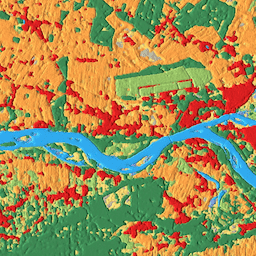
Dynamic World は、10 m の準リアルタイム（NRT）の土地利用/土地被覆（LULC）データセットで、9 つのクラスのクラス確率とラベル情報が含まれています。

Dynamic World の予測は、2015 年 6 月 27 日から現在までの Sentinel-2 L1C コレクションで利用できます。Sentinel-2 の再訪頻度は、緯度によって 2 ～ 5 日です。Dynamic World の予測は、CLOUDY_PIXEL_PERCENTAGE <= 35% の Sentinel-2 L1C 画像に対して生成されます。予測は、S2 Cloud Probability、Cloud Displacement Index、Directional Distance Transform を組み合わせて、雲と雲の影を削除するようにマスクされます。

Dynamic World コレクションの画像の名前は、派生元の個々の Sentinel-2 L1C アセット名と一致します。例:

ee.Image('COPERNICUS/S2/20160711T084022_20160711T084751_T35PKT')

には、 ee.Image('GOOGLE/DYNAMICWORLD/V1/20160711T084022_20160711T084751_T35PKT') という名前の対応する Dynamic World 画像があります。

[label] バンドを除くすべての確率バンドの合計は 1 です。

Dynamic World データセットの詳細、合成の生成、地域統計の計算、時系列の操作の例については、Dynamic World の概要チュートリアルシリーズをご覧ください。

Dynamic World のクラス推定は、小さな移動ウィンドウの空間コンテキストを使用して単一の画像から導出されるため、作物のようないくつかの土地被覆で定義される予測された土地被覆のトップ 1 の「確率」は、明らかな識別特徴がない場合、比較的低くなる可能性があります。乾燥した気候、砂、太陽光の反射などの高反射面でも、この現象が発生する可能性があります。

Dynamic World クラスに確実に属するピクセルのみを選択するには、トップ 1 の予測の推定「確率」を閾値処理して Dynamic World の出力をマスクすることをおすすめします。

バンド

バンド

ピクセルサイズ: 10 メートル（すべてのバンド）

名前	最大	ピクセルサイズ	説明
`water`	1	10 メートル	水による完全な被覆の推定確率
`trees`	1	10 メートル	木による完全な被覆の推定確率
`grass`	1	10 メートル	草による完全な被覆の推定確率
`flooded_vegetation`	1	10 メートル	浸水した植生による完全な被覆の推定確率
`crops`	1	10 メートル	作物による完全な被覆の推定確率
`shrub_and_scrub`	1	10 メートル	低木と低木による完全な被覆の推定確率
`built`	1	10 メートル	建物による完全な被覆の推定確率
`bare`	1	10 メートル	裸地による完全な被覆の推定確率
`snow_and_ice`	1	10 メートル	雪と氷による完全な被覆の推定確率
`label`	8	10 メートル	推定確率が最も高いバンドのインデックス

ラベルクラステーブル

値	色	説明
0	#419bdf	水
1	#397d49	木
2	#88b053	草
3	#7a87c6	flooded_vegetation
4	#e49635	作物
5	#dfc35a	shrub_and_scrub
6	#c4281b	建物
7	#a59b8f	裸地
8	#b39fe1	snow_and_ice

画像プロパティ検出

画像プロパティ検出

名前	型	説明
dynamicworld_algorithm_version	STRING	画像の生成に使用された Dynamic World モデルと推論プロセスを一意に識別するバージョン文字列。
qa_algorithm_version	STRING	画像の生成に使用されたクラウドマスク処理を一意に識別するバージョン文字列。

利用規約

利用規約

このデータセットは CC-BY 4.0 のライセンスで提供されており、次の帰属表示が必要です。「このデータセットは、ナショナルジオグラフィック協会と World Resources Institute が協力して Google が Dynamic World プロジェクトのために作成したものです。」

修正された Copernicus Sentinel データ [2015 年～現在] が含まれています。 Sentinel データの法的通知をご覧ください。

引用

Brown, C.F., Brumby, S.P., Guzder-Williams, B. et al. Dynamic World, Near real-time global 10 m land use land cover mapping. Sci Data 9, 251 (2022). doi:10.1038/s41597-022-01307-4

DOI

https://doi.org/10.1038/s41597-022-01307-4

Earth Engine で探索する

コードエディタ（JavaScript）

// Construct a collection of corresponding Dynamic World and Sentinel-2 for
// inspection. Filter by region and date.
var START = ee.Date('2021-04-02');
var END = START.advance(1, 'day');

var colFilter = ee.Filter.and(
    ee.Filter.bounds(ee.Geometry.Point(20.6729, 52.4305)),
    ee.Filter.date(START, END));

var dwCol = ee.ImageCollection('GOOGLE/DYNAMICWORLD/V1').filter(colFilter);
var s2Col = ee.ImageCollection('COPERNICUS/S2_HARMONIZED');

// Link DW and S2 source images.
var linkedCol = dwCol.linkCollection(s2Col, s2Col.first().bandNames());

// Get example DW image with linked S2 image.
var linkedImg = ee.Image(linkedCol.first());

// Create a visualization that blends DW class label with probability.
// Define list pairs of DW LULC label and color.
var CLASS_NAMES = [
    'water', 'trees', 'grass', 'flooded_vegetation', 'crops',
    'shrub_and_scrub', 'built', 'bare', 'snow_and_ice'];

var VIS_PALETTE = [
    '419bdf', '397d49', '88b053', '7a87c6', 'e49635', 'dfc35a', 'c4281b',
    'a59b8f', 'b39fe1'];

// Create an RGB image of the label (most likely class) on [0, 1].
var dwRgb = linkedImg
    .select('label')
    .visualize({min: 0, max: 8, palette: VIS_PALETTE})
    .divide(255);

// Get the most likely class probability.
var top1Prob = linkedImg.select(CLASS_NAMES).reduce(ee.Reducer.max());

// Create a hillshade of the most likely class probability on [0, 1];
var top1ProbHillshade =
    ee.Terrain.hillshade(top1Prob.multiply(100))
    .divide(255);

// Combine the RGB image with the hillshade.
var dwRgbHillshade = dwRgb.multiply(top1ProbHillshade);

// Display the Dynamic World visualization with the source Sentinel-2 image.
Map.setCenter(20.6729, 52.4305, 12);
Map.addLayer(
    linkedImg, {min: 0, max: 3000, bands: ['B4', 'B3', 'B2']}, 'Sentinel-2 L1C');
Map.addLayer(
    dwRgbHillshade, {min: 0, max: 0.65}, 'Dynamic World V1 - label hillshade');

Python の設定

Python API と geemap を使用したインタラクティブな開発については、 Python 環境のページをご覧ください。

import ee
import geemap.core as geemap

Colab（Python）

# Construct a collection of corresponding Dynamic World and Sentinel-2 for
# inspection. Filter by region and date.
START = ee.Date('2021-04-02')
END = START.advance(1, 'day')

col_filter = ee.Filter.And(
    ee.Filter.bounds(ee.Geometry.Point(20.6729, 52.4305)),
    ee.Filter.date(START, END),
)

dw_col = ee.ImageCollection('GOOGLE/DYNAMICWORLD/V1').filter(col_filter)
s2_col = ee.ImageCollection('COPERNICUS/S2_HARMONIZED');

# Link DW and S2 source images.
linked_col = dw_col.linkCollection(s2_col, s2_col.first().bandNames());

# Get example DW image with linked S2 image.
linked_image = ee.Image(linked_col.first())

# Create a visualization that blends DW class label with probability.
# Define list pairs of DW LULC label and color.
CLASS_NAMES = [
    'water',
    'trees',
    'grass',
    'flooded_vegetation',
    'crops',
    'shrub_and_scrub',
    'built',
    'bare',
    'snow_and_ice',
]

VIS_PALETTE = [
    '419bdf',
    '397d49',
    '88b053',
    '7a87c6',
    'e49635',
    'dfc35a',
    'c4281b',
    'a59b8f',
    'b39fe1',
]

# Create an RGB image of the label (most likely class) on [0, 1].
dw_rgb = (
    linked_image.select('label')
    .visualize(min=0, max=8, palette=VIS_PALETTE)
    .divide(255)
)

# Get the most likely class probability.
top1_prob = linked_image.select(CLASS_NAMES).reduce(ee.Reducer.max())

# Create a hillshade of the most likely class probability on [0, 1]
top1_prob_hillshade = ee.Terrain.hillshade(top1_prob.multiply(100)).divide(255)

# Combine the RGB image with the hillshade.
dw_rgb_hillshade = dw_rgb.multiply(top1_prob_hillshade)

# Display the Dynamic World visualization with the source Sentinel-2 image.
m = geemap.Map()
m.set_center(20.6729, 52.4305, 12)
m.add_layer(
    linked_image,
    {'min': 0, 'max': 3000, 'bands': ['B4', 'B3', 'B2']},
    'Sentinel-2 L1C',
)
m.add_layer(
    dw_rgb_hillshade,
    {'min': 0, 'max': 0.65},
    'Dynamic World V1 - label hillshade',
)
m

コードエディタで開く

Dynamic World V1

Dynamic World は、10 m の準リアルタイム（NRT）の土地利用/土地被覆（LULC）データセットで、9 つのクラスのクラス確率とラベル情報が含まれています。Dynamic World の予測は、2015 年 6 月 27 日から現在までの Sentinel-2 L1C コレクションで利用できます。Sentinel-2 の再訪頻度は、緯度によって 2 ～ 5 日です。Dynamic World …

GOOGLE/DYNAMICWORLD/V1, global,google,landcover,landuse,landuse-landcover,nrt,sentinel2-derived

2015-06-27T00:00:00Z/2026-03-26T01:59:44.220000Z

-90 -180 90 180

Google Earth Engine

https://developers.google.com/earth-engine/datasets

Dynamic World V1 コレクションでコンテンツを整理 必要に応じて、コンテンツの保存と分類を行います。

説明

バンド

画像プロパティ検出

利用規約

引用

DOI

Earth Engine で探索する

コードエディタ（JavaScript）

Colab（Python）

Dynamic World V1