
1. 事前準備
在這個程式碼研究室中,您將使用卷積將馬匹和人類的圖片分類。您將在這項研究室中使用 TensorFlow,建立 CNN 來訓練辨識辨識馬匹和人類的圖片,並將這些模型分類。
事前準備
如果您從未透過 TensorFlow 建構卷積,建議完成建構卷積和執行集區程式碼研究室。在本練習中,我們導入卷積和集區,並建構卷積類神經網路 (CNN) 來強化電腦視覺技術,藉此探討如何提升電腦的辨識能力。
您將會瞭解的內容
- 如何訓練電腦辨識圖片中主題的特色
建構項目
- 一個卷積類神經網路,可用來區分馬匹或人類的相片
軟硬體需求
您可以找到在 Colab 中執行的其他程式碼研究室程式碼。
你也必須安裝 TensorFlow,以及先前在程式碼研究室安裝的程式庫。
2. 開始使用:取得資料
為此,您需要建立一個馬匹或是人類分類,用來判斷指定圖片中是否包含馬匹或是人類,然後透過網路訓練辨識辨識哪些特徵。在進行訓練之前,您必須先處理一些資料。
首先,請下載資料:
!wget --no-check-certificate https://storage.googleapis.com/laurencemoroney-blog.appspot.com/horse-or-human.zip -O /tmp/horse-or-human.zip
下列 Python 程式碼會使用 OS 程式庫使用作業系統程式庫,讓您存取檔案系統和 ZIP 檔案程式庫,進而解壓縮資料。
import os
import zipfile

local_zip = '/tmp/horse-or-human.zip'
zip_ref = zipfile.ZipFile(local_zip, 'r')
zip_ref.extractall('/tmp/horse-or-human')
zip_ref.close()
ZIP 檔案內容已解壓縮至基本目錄 /tmp/horse-or-human,其中包含馬匹和人類子目錄。
簡單來說,訓練集是用來告知類神經網路模型的資料,也就是「馬匹的外貌」。和「人類的樣子」
3. 使用 ImageGenerator 來標記及準備資料
您未明確將圖片標示為馬匹或人類。
系統稍後會顯示「ImageDataGenerator」。這會讀取子目錄中的圖片,並自動為該子目錄命名。例如,您有一個訓練目錄,其中包含馬匹目錄以及人類目錄。ImageDataGenerator 會為圖片加上合適的標籤,以減少編碼步驟。
請定義每個目錄。
# Directory with our training horse pictures
train_horse_dir = os.path.join('/tmp/horse-or-human/horses')

# Directory with our training human pictures
train_human_dir = os.path.join('/tmp/horse-or-human/humans')
現在,請查看檔案名稱和人類訓練目錄中的檔案名稱:
train_horse_names = os.listdir(train_horse_dir)
print(train_horse_names[:10])
train_human_names = os.listdir(train_human_dir)
print(train_human_names[:10])
請在目錄中找出馬匹和人類圖片的總數:
print('total training horse images:', len(os.listdir(train_horse_dir)))
print('total training human images:', len(os.listdir(train_human_dir)))
4. 探索資料
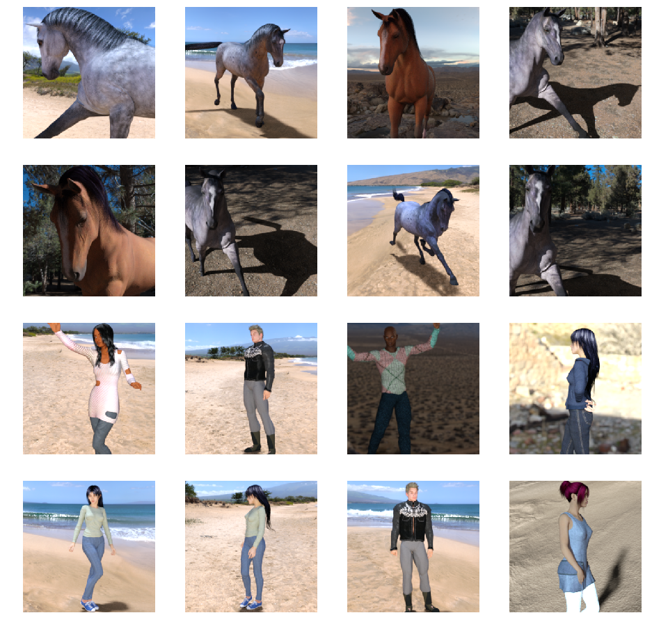
請看幾張相片,看看這些文字的效果。
首先,設定 matplot 參數:
%matplotlib inline

import matplotlib.pyplot as plt
import matplotlib.image as mpimg

# Parameters for our graph; we'll output images in a 4x4 configuration
nrows = 4
ncols = 4

# Index for iterating over images
pic_index = 0
現在,您可以看到一批八張馬的圖片和八張人類圖片。您每次可以重新執行儲存格,讓系統顯示最新的批次項目。
# Set up matplotlib fig, and size it to fit 4x4 pics
fig = plt.gcf()
fig.set_size_inches(ncols * 4, nrows * 4)

pic_index += 8
next_horse_pix = [os.path.join(train_horse_dir, fname)
                for fname in train_horse_names[pic_index-8:pic_index]]
next_human_pix = [os.path.join(train_human_dir, fname)
                for fname in train_human_names[pic_index-8:pic_index]]

for i, img_path in enumerate(next_horse_pix+next_human_pix):
  # Set up subplot; subplot indices start at 1
  sp = plt.subplot(nrows, ncols, i + 1)
  sp.axis('Off') # Don't show axes (or gridlines)

  img = mpimg.imread(img_path)
  plt.imshow(img)

plt.show()
以下圖片範例呈現不同姿勢和方向的馬和人類:
5. 定義模型
開始定義模型。
首先,匯入 TensorFlow:
import tensorflow as tf
然後,加入卷積層並分割最終結果,以建立密集連結的圖層。最後,新增密集的圖層。
請注意,由於您面臨兩個類別的分類問題 (「二元分類」問題),因此您的網路將會以「sigmoid 啟用」做為結尾,讓網路的輸出將是介於 0 和 1 之間的純量,用來編碼目前圖片為第 1 類 (而非第 0 類) 的機率。
model = tf.keras.models.Sequential([
    # Note the input shape is the desired size of the image 300x300 with 3 bytes color
    # This is the first convolution
    tf.keras.layers.Conv2D(16, (3,3), activation='relu', input_shape=(300, 300, 3)),
    tf.keras.layers.MaxPooling2D(2, 2),
    # The second convolution
    tf.keras.layers.Conv2D(32, (3,3), activation='relu'),
    tf.keras.layers.MaxPooling2D(2,2),
    # The third convolution
    tf.keras.layers.Conv2D(64, (3,3), activation='relu'),
    tf.keras.layers.MaxPooling2D(2,2),
    # The fourth convolution
    tf.keras.layers.Conv2D(64, (3,3), activation='relu'),
    tf.keras.layers.MaxPooling2D(2,2),
    # The fifth convolution
    tf.keras.layers.Conv2D(64, (3,3), activation='relu'),
    tf.keras.layers.MaxPooling2D(2,2),
    # Flatten the results to feed into a DNN
    tf.keras.layers.Flatten(),
    # 512 neuron hidden layer
    tf.keras.layers.Dense(512, activation='relu'),
    # Only 1 output neuron. It will contain a value from 0-1 where 0 for 1 class ('horses') and 1 for the other ('humans')
    tf.keras.layers.Dense(1, activation='sigmoid')
])
model.summary() 方法呼叫會列印網路的摘要。
model.summary()
你可以在這裡查看結果:
Layer (type)                 Output Shape              Param #
=================================================================
conv2d (Conv2D)              (None, 298, 298, 16)      448
_________________________________________________________________
max_pooling2d (MaxPooling2D) (None, 149, 149, 16)      0
_________________________________________________________________
conv2d_1 (Conv2D)            (None, 147, 147, 32)      4640
_________________________________________________________________
max_pooling2d_1 (MaxPooling2 (None, 73, 73, 32)        0
_________________________________________________________________
conv2d_2 (Conv2D)            (None, 71, 71, 64)        18496
_________________________________________________________________
max_pooling2d_2 (MaxPooling2 (None, 35, 35, 64)        0
_________________________________________________________________
conv2d_3 (Conv2D)            (None, 33, 33, 64)        36928
_________________________________________________________________
max_pooling2d_3 (MaxPooling2 (None, 16, 16, 64)        0
_________________________________________________________________
conv2d_4 (Conv2D)            (None, 14, 14, 64)        36928
_________________________________________________________________
max_pooling2d_4 (MaxPooling2 (None, 7, 7, 64)          0
_________________________________________________________________
flatten (Flatten)            (None, 3136)              0
_________________________________________________________________
dense (Dense)                (None, 512)               1606144
_________________________________________________________________
dense_1 (Dense)              (None, 1)                 513
=================================================================
Total params: 1,704,097
Trainable params: 1,704,097
Non-trainable params: 0
輸出形狀欄會顯示每個連續圖層的特徵圖大小變化。卷積層因為填充程度而縮減了特徵的大小,而每個集區層的分層大小也減少了一半。
6. 編譯模型
接著,設定模型訓練的規格。使用 binary_crossentropy 損失的訓練模型,因為模型是二元分類問題,而最終啟用是 Sigmoid。(如要瞭解損失指標的複習情形,請參閱深入研究機器學習)。使用 rmsprop 最佳化工具,學習率為 0.001。在訓練過程中,監控分類準確度。
from tensorflow.keras.optimizers import RMSprop

model.compile(loss='binary_crossentropy',
              optimizer=RMSprop(lr=0.001),
              metrics=['acc'])
7. 從發電機訓練模型
設定資料產生器以讀取來源資料夾中的圖片、將其轉換為 浮點數 32 張張量,然後將這些濾鏡 (連同標籤的標籤) 傳送到您的網路。
您將擁有一個用於訓練映像檔的產生器,還有一個用於驗證圖片的產生器。您的產生器會產生一批大小為 300x300 的圖片和其標籤 (二進位)。
如您所知,進入類神經網路的資料通常都會經過正規化,讓該網路更容易處理。(將原始像素提交至 CNN 是很常見的情況)。在您的情況下,您將通過將像素值幀化到 [0, 1] 範圍內(首先所有值都在 [0, 255] 範圍內),然後將您的圖像進行預先處理。
在 Keras 中,您可以使用 keras.preprocessing.image.ImageDataGenerator 類別透過 rescale 參數完成此作業。這個 ImageDataGenerator 類別可讓您以 .flow (data, label) 或 .flow_from_directory(directory) 將擴增圖片批次(及其標籤) 的產生器化為執行個體。這些發電機可與 Keras 模型方法搭配使用,以接受資料產生器做為輸入來源:fit_generator、evaluate_generator 和 predict_generator。
from tensorflow.keras.preprocessing.image import ImageDataGenerator

# All images will be rescaled by 1./255
train_datagen = ImageDataGenerator(rescale=1./255)

# Flow training images in batches of 128 using train_datagen generator
train_generator = train_datagen.flow_from_directory(
        '/tmp/horse-or-human/',  # This is the source directory for training images
        target_size=(300, 300),  # All images will be resized to 150x150
        batch_size=128,
        # Since we use binary_crossentropy loss, we need binary labels
        class_mode='binary')
8. 進行訓練
訓練 15 個訓練週期。(可能需要幾分鐘的時間才能執行)。
history = model.fit(
      train_generator,
      steps_per_epoch=8,
      epochs=15,
      verbose=1)
記下每個訓練週期的值。
「Loss」和「Accuracy」是很好的訓練進度。它會猜測訓練資料的分類,然後根據已知標籤來評估資料,然後計算結果。精確度是正確猜測的部分。
Epoch 1/15
9/9 [==============================] - 9s 1s/step - loss: 0.8662 - acc: 0.5151
Epoch 2/15
9/9 [==============================] - 8s 927ms/step - loss: 0.7212 - acc: 0.5969
Epoch 3/15
9/9 [==============================] - 8s 921ms/step - loss: 0.6612 - acc: 0.6592
Epoch 4/15
9/9 [==============================] - 8s 925ms/step - loss: 0.3135 - acc: 0.8481
Epoch 5/15
9/9 [==============================] - 8s 919ms/step - loss: 0.4640 - acc: 0.8530
Epoch 6/15
9/9 [==============================] - 8s 896ms/step - loss: 0.2306 - acc: 0.9231
Epoch 7/15
9/9 [==============================] - 8s 915ms/step - loss: 0.1464 - acc: 0.9396
Epoch 8/15
9/9 [==============================] - 8s 935ms/step - loss: 0.2663 - acc: 0.8919
Epoch 9/15
9/9 [==============================] - 8s 883ms/step - loss: 0.0772 - acc: 0.9698
Epoch 10/15
9/9 [==============================] - 9s 951ms/step - loss: 0.0403 - acc: 0.9805
Epoch 11/15
9/9 [==============================] - 8s 891ms/step - loss: 0.2618 - acc: 0.9075
Epoch 12/15
9/9 [==============================] - 8s 902ms/step - loss: 0.0434 - acc: 0.9873
Epoch 13/15
9/9 [==============================] - 8s 904ms/step - loss: 0.0187 - acc: 0.9932
Epoch 14/15
9/9 [==============================] - 9s 951ms/step - loss: 0.0974 - acc: 0.9649
Epoch 15/15
9/9 [==============================] - 8s 877ms/step - loss: 0.2859 - acc: 0.9338
9. 測試模型
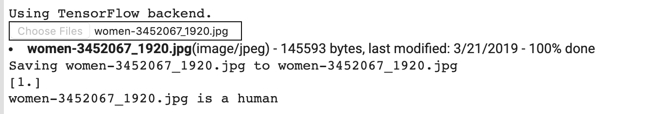
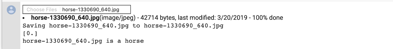
現在使用模型進行預測。從程式碼中選擇一個或多個檔案。然後會上傳模型,然後透過模型執行,指出該物件是馬匹或是人類。
您可以將網際網路上的圖片下載到檔案系統,立即體驗!請注意,您可能會發現訓練程序產生許多錯誤,即使訓練的準確率超過 99%。
不過,由於所謂的「過度配適」,因此類神經網路是用有限的資料進行訓練 (每個類別僅有約 500 張圖片)。因此,如果能辨識訓練集裡的圖片,就很適合使用它,但若不是訓練集內的圖片,可能會大失成功。
這已經是一個資料點,可以證明你訓練的資料越多,最終的網路設定就越好。
雖然有許多資料 (例如稱為圖片擴增等) 的資料有限,但您還是可以透過許多技巧改善訓練,但這不在程式碼研究室所涵蓋的範圍之外。
import numpy as np
from google.colab import files
from keras.preprocessing import image

uploaded = files.upload()

for fn in uploaded.keys():

  # predicting images
  path = '/content/' + fn
  img = image.load_img(path, target_size=(300, 300))
  x = image.img_to_array(img)
  x = np.expand_dims(x, axis=0)

  images = np.vstack([x])
  classes = model.predict(images, batch_size=10)
  print(classes[0])
  if classes[0]>0.5:
    print(fn + " is a human")
  else:
    print(fn + " is a horse")
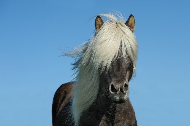
舉例來說,假設您想使用這個圖片進行測試:

以下是 Colab 製作的內容:
儘管它是卡通圖像,但仍能正確分類。
以下圖片也正確分類:
嘗試自行設計圖片並探索!
10. 以視覺化方式呈現中間表示法
為瞭解 CNN 所學到的特徵,有一項有趣的功能可以視覺化呈現輸入在 CNN 過程中的轉換效果。
從訓練集中選擇隨機圖片,然後產生一個圖表,其中每一列是圖層的輸出,而資料列中的每個圖片都是該輸出特徵對應的特定篩選條件。重新執行該儲存格,為各種訓練圖片產生中繼表示法。
import numpy as np
import random
from tensorflow.keras.preprocessing.image import img_to_array, load_img

# Let's define a new Model that will take an image as input, and will output
# intermediate representations for all layers in the previous model after
# the first.
successive_outputs = [layer.output for layer in model.layers[1:]]
#visualization_model = Model(img_input, successive_outputs)
visualization_model = tf.keras.models.Model(inputs = model.input, outputs = successive_outputs)
# Let's prepare a random input image from the training set.
horse_img_files = [os.path.join(train_horse_dir, f) for f in train_horse_names]
human_img_files = [os.path.join(train_human_dir, f) for f in train_human_names]
img_path = random.choice(horse_img_files + human_img_files)

img = load_img(img_path, target_size=(300, 300))  # this is a PIL image
x = img_to_array(img)  # Numpy array with shape (150, 150, 3)
x = x.reshape((1,) + x.shape)  # Numpy array with shape (1, 150, 150, 3)

# Rescale by 1/255
x /= 255

# Let's run our image through our network, thus obtaining all
# intermediate representations for this image.
successive_feature_maps = visualization_model.predict(x)

# These are the names of the layers, so can have them as part of our plot
layer_names = [layer.name for layer in model.layers]

# Now let's display our representations
for layer_name, feature_map in zip(layer_names, successive_feature_maps):
  if len(feature_map.shape) == 4:
    # Just do this for the conv / maxpool layers, not the fully-connected layers
    n_features = feature_map.shape[-1]  # number of features in feature map
    # The feature map has shape (1, size, size, n_features)
    size = feature_map.shape[1]
    # We will tile our images in this matrix
    display_grid = np.zeros((size, size * n_features))
    for i in range(n_features):
      # Postprocess the feature to make it visually palatable
      x = feature_map[0, :, :, i]
      x -= x.mean()
      if x.std()>0:
        x /= x.std()
      x *= 64
      x += 128
      x = np.clip(x, 0, 255).astype('uint8')
      # We'll tile each filter into this big horizontal grid
      display_grid[:, i * size : (i + 1) * size] = x
    # Display the grid
    scale = 20. / n_features
    plt.figure(figsize=(scale * n_features, scale))
    plt.title(layer_name)
    plt.grid(False)
    plt.imshow(display_grid, aspect='auto', cmap='viridis')
以下是範例結果:
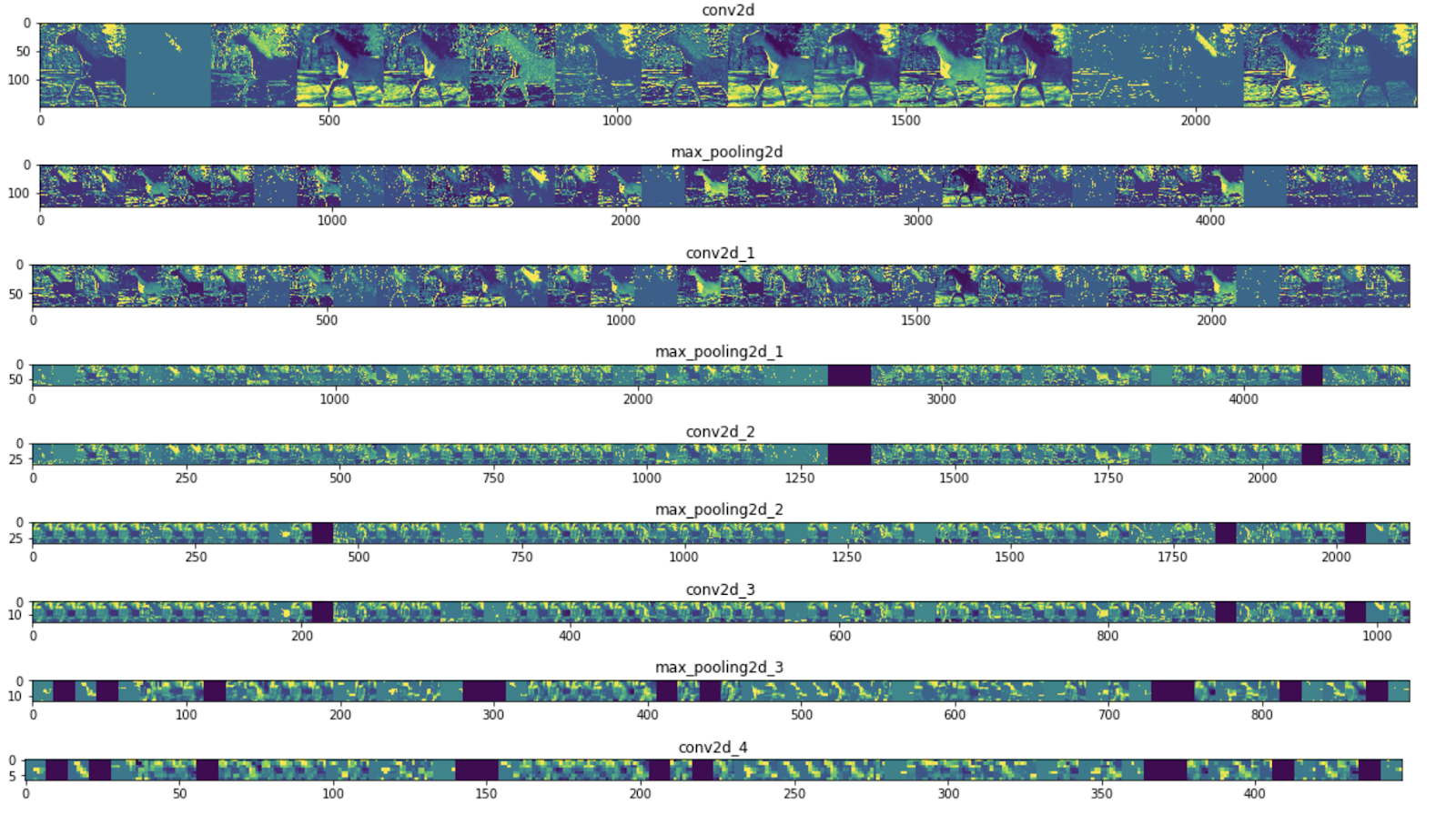
如您所見,您可以從圖片的原始像素開始逐漸變為精簡。代表下游的重點在於網路所關注的部分,並顯示「啟用」的較少與較少功能。大部分都設為零。這就是所謂的 sparsity。表示法式稀疏度是深度學習的關鍵功能,
這些表示法在圖片的原始像素相關資訊上越來越少,但圖片類別的相關資訊越來越精細。您可以將 CNN (或一般網路) 視為資訊蒸餾管道。
11. 恭喜
你學會使用 CNN 強化複雜的圖片。要進一步瞭解如何進一步強化您的電腦視覺模型,請參閱將大型類神經網路 (CNN) 與大型資料集搭配使用,以免過度配適。