
1. 事前準備
在本程式碼研究室中,您將瞭解捲積,以及這項技術在電腦視覺情境中為何如此強大。
在先前的程式碼研究室中,您建立了簡單的深層類神經網路 (DNN),用於時尚商品的電腦視覺。這項限制是因為圖片中只能有衣物,而且必須置中。
當然,這並非實際情況。您會希望 DNN 能夠辨識圖片中的服飾,即使圖片中還有其他物體,或服飾並非位於正中央。為此,您需要使用捲積。
必要條件
本程式碼研究室以先前兩項作業為基礎,分別是「向機器學習的『Hello, World』問好」和「建構電腦視覺模型」。請先完成這些程式碼研究室,再繼續操作。
課程內容
- 什麼是捲積
- 如何建立特徵地圖
- 什麼是共用?
建構項目
- 圖片的特徵地圖
軟硬體需求
您可以在 Colab 中執行本程式碼研究室的其餘程式碼。
您也需要安裝 TensorFlow,以及在先前的程式碼研究室中安裝的程式庫。
2. 什麼是捲積?
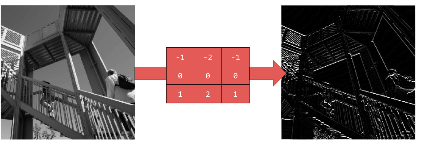
卷積是一種濾波器,會套用至圖片、加以處理,再從中擷取重要特徵。
假設你有一張圖片,裡面的人穿著運動鞋。你會如何偵測圖片中是否有運動鞋?為了讓程式「看見」運動鞋的圖像,您必須擷取重要特徵,並模糊處理不必要的特徵。這就是所謂的「功能對應」。
理論上,功能對應程序很簡單。您會掃描圖片中的每個像素,然後查看相鄰像素。然後將這些像素的值乘以篩選器中的對等權重。
例如:
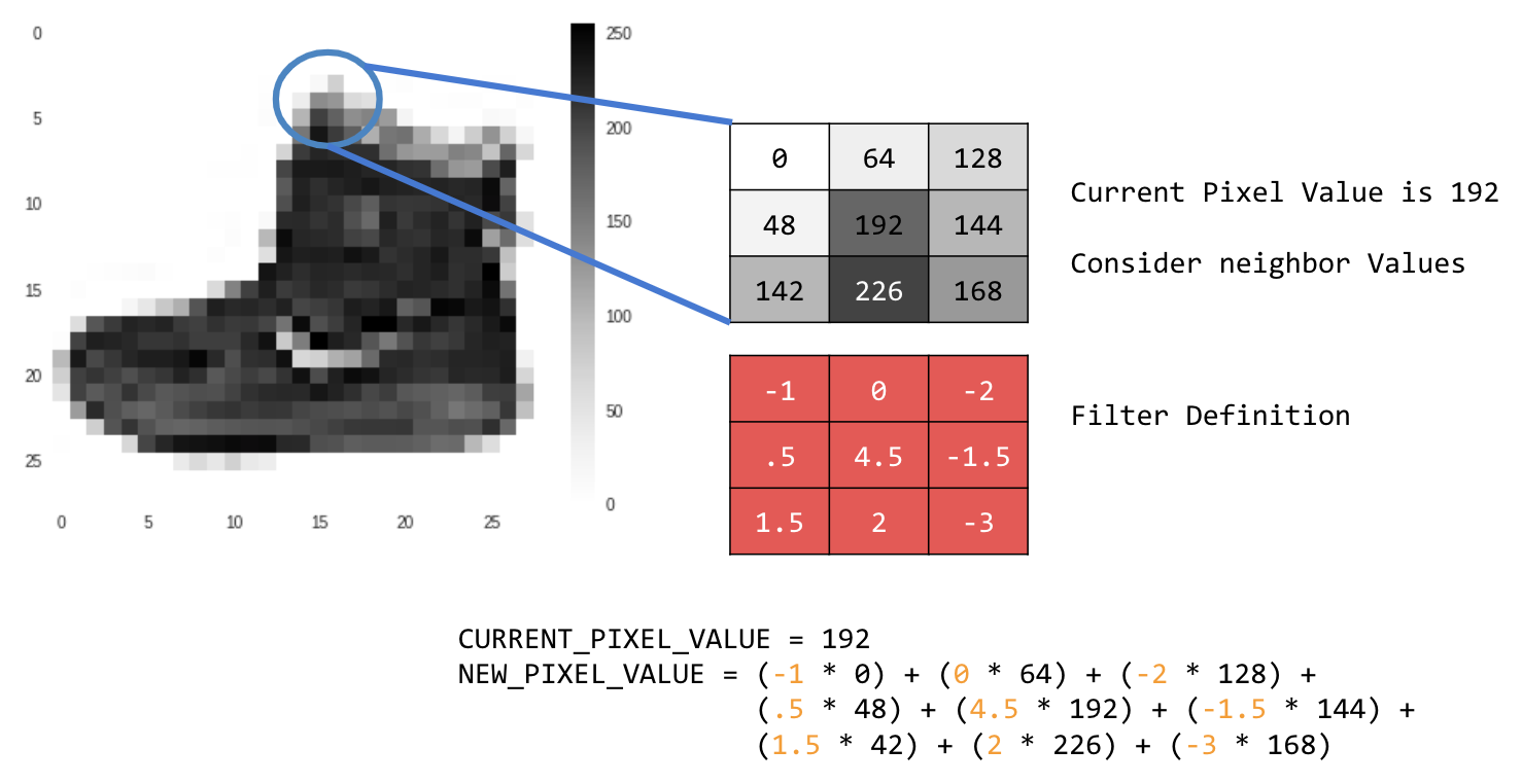
在本例中,系統會指定 3x3 捲積矩陣或圖片核心。
目前的像素值為 192。您可以查看鄰近值、將這些值乘以篩選器中指定的值,然後將新像素值設為最終金額,藉此計算新像素的值。
現在,請建立 2D 灰階圖片的基本捲積,瞭解捲積的運作方式。
您將使用 SciPy 的 ascent 圖片進行示範。這張內建圖片的線條和角度都很漂亮。
3. 開始編寫程式碼
首先,請匯入一些 Python 程式庫和 ascent 圖片:
import cv2
import numpy as np
from scipy import misc
i = misc.ascent()
接著,使用 Pyplot 程式庫 matplotlib 繪製圖片,瞭解圖片的樣子:
import matplotlib.pyplot as plt
plt.grid(False)
plt.gray()
plt.axis('off')
plt.imshow(i)
plt.show()
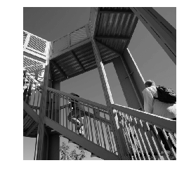
你可以看到這是樓梯間的圖片。你可以嘗試並隔離許多功能。例如,有明顯的垂直線。
圖片會儲存為 NumPy 陣列,因此只要複製該陣列,就能建立轉換後的圖片。size_x 和 size_y 變數會保留圖片的尺寸,方便您稍後進行迴圈。
i_transformed = np.copy(i)
size_x = i_transformed.shape[0]
size_y = i_transformed.shape[1]
4. 建立捲積矩陣
首先,請將捲積矩陣 (或核心) 設為 3x3 陣列:
# This filter detects edges nicely
# It creates a filter that only passes through sharp edges and straight lines.
# Experiment with different values for fun effects.
#filter = [ [0, 1, 0], [1, -4, 1], [0, 1, 0]]
# A couple more filters to try for fun!
filter = [ [-1, -2, -1], [0, 0, 0], [1, 2, 1]]
#filter = [ [-1, 0, 1], [-2, 0, 2], [-1, 0, 1]]
 # If all the digits in the filter don't add up to 0 or 1, you
# should probably do a weight to get it to do so
# so, for example, if your weights are 1,1,1 1,2,1 1,1,1
# They add up to 10, so you would set a weight of .1 if you want to normalize them
weight  = 1
現在,請計算輸出像素。疊代圖片,保留 1 像素的邊界,然後將目前像素的每個鄰近像素乘以篩選器中定義的值。
也就是說,目前像素上方和左側的鄰近像素會乘以篩選器左上方的項目。然後將結果乘以權重,並確保結果介於 0 到 255 之間。
最後,將新值載入轉換後的圖片:
for x in range(1,size_x-1):
  for y in range(1,size_y-1):
      output_pixel = 0.0
      output_pixel = output_pixel + (i[x - 1, y-1] * filter[0][0])
      output_pixel = output_pixel + (i[x, y-1] * filter[0][1])
      output_pixel = output_pixel + (i[x + 1, y-1] * filter[0][2])
      output_pixel = output_pixel + (i[x-1, y] * filter[1][0])
      output_pixel = output_pixel + (i[x, y] * filter[1][1])
      output_pixel = output_pixel + (i[x+1, y] * filter[1][2])
      output_pixel = output_pixel + (i[x-1, y+1] * filter[2][0])
      output_pixel = output_pixel + (i[x, y+1] * filter[2][1])
      output_pixel = output_pixel + (i[x+1, y+1] * filter[2][2])
      output_pixel = output_pixel * weight
      if(output_pixel<0):
        output_pixel=0
      if(output_pixel>255):
        output_pixel=255
      i_transformed[x, y] = output_pixel
5. 查看結果
現在,繪製圖片,看看將濾鏡傳遞至圖片的效果:
# Plot the image. Note the size of the axes -- they are 512 by 512
plt.gray()
plt.grid(False)
plt.imshow(i_transformed)
#plt.axis('off')
plt.show()
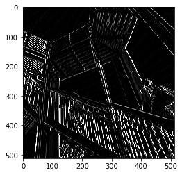
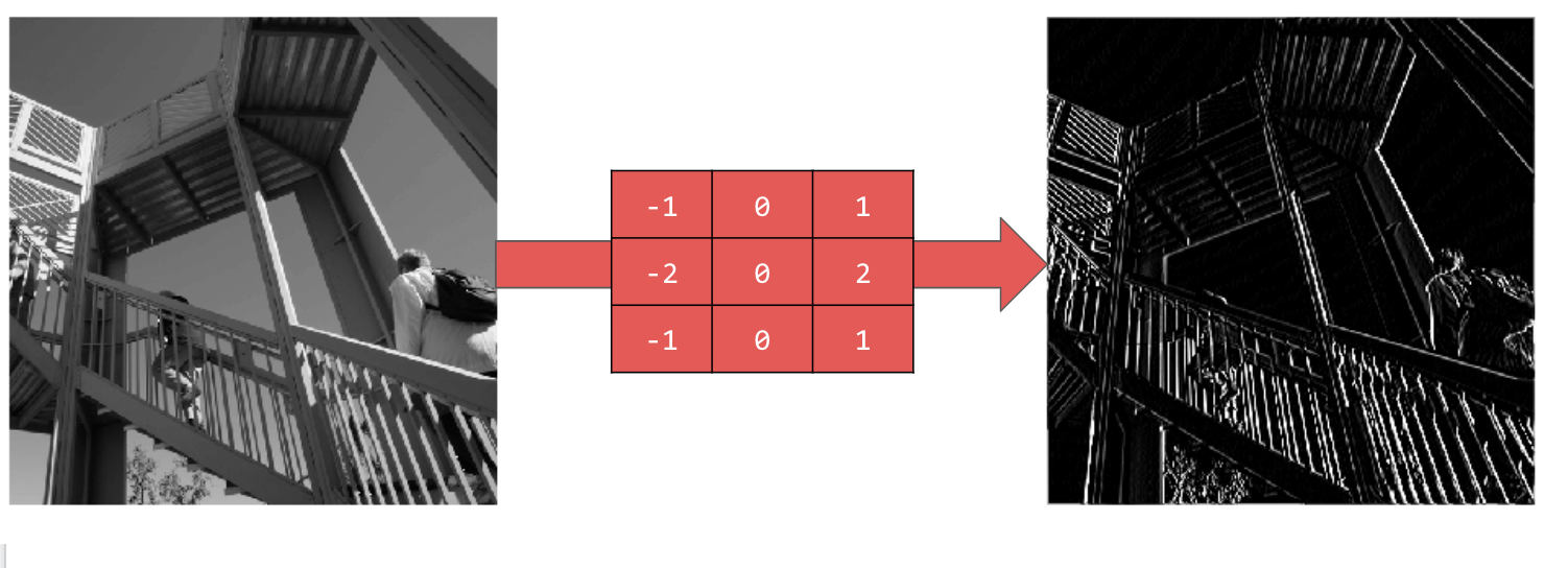
請參考下列濾鏡值及其對圖片的影響。
使用 [-1,0,1,-2,0,2,-1,0,1] 可產生非常強烈的垂直線:
使用 [-1,-2,-1,0,0,0,1,2,1] 可產生水平線:
探索不同的價值!此外,你也可以嘗試不同大小的濾鏡,例如 5x5 或 7x7。
6. 瞭解集區
現在您已找出圖片的重要特徵,接下來該怎麼做?如何使用產生的特徵地圖分類圖片?
與捲積類似,集區化有助於偵測特徵。匯集層可減少圖片中的整體資訊量,同時保留偵測到的特徵。
集區有多種不同類型,但您會使用稱為「最大 (Max) 集區」的類型。
逐一疊代圖片,並在每個點考慮像素及其右側、下方和右下方的直接鄰近像素。從中選取最大值 (因此為 max 集區),然後載入新圖片。因此,新圖片的大小會是舊圖片的四分之一。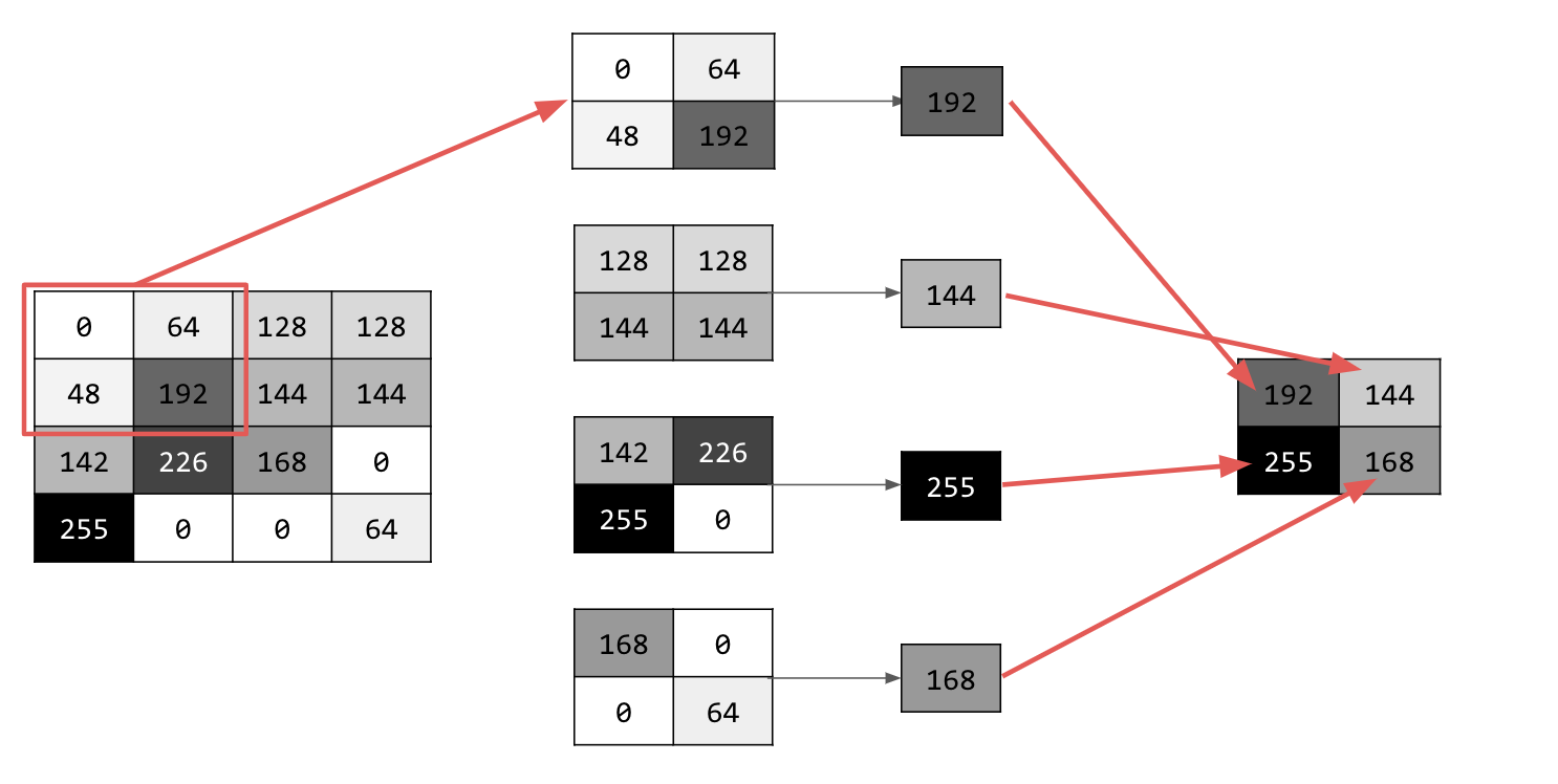
7. 編寫集區程式碼
下列程式碼會顯示 (2, 2) 集區化。執行指令碼,查看輸出內容。
你會發現,雖然圖片只有原始大小的四分之一,但所有特徵都保留下來了。
new_x = int(size_x/2)
new_y = int(size_y/2)
newImage = np.zeros((new_x, new_y))
for x in range(0, size_x, 2):
  for y in range(0, size_y, 2):
    pixels = []
    pixels.append(i_transformed[x, y])
    pixels.append(i_transformed[x+1, y])
    pixels.append(i_transformed[x, y+1])
    pixels.append(i_transformed[x+1, y+1])
    pixels.sort(reverse=True)
    newImage[int(x/2),int(y/2)] = pixels[0]

# Plot the image. Note the size of the axes -- now 256 pixels instead of 512
plt.gray()
plt.grid(False)
plt.imshow(newImage)
#plt.axis('off')
plt.show()
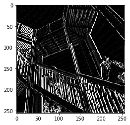
請注意該圖的軸。圖片現在是 256x256,只有原始大小的四分之一,但即使圖片資料較少,偵測到的特徵仍有所提升。
8. 恭喜
您已建構第一個電腦視覺模型!如要瞭解如何進一步提升電腦視覺模型效能,請參閱「建構卷積類神經網路 (CNN),提升電腦視覺效能」。