
1. 始める前に
この Codelab では、畳み込みを使って馬と人間の画像を分類します。このラボでは、TensorFlow を使用して、馬と人間の画像を認識して分類するためのトレーニング済み CNN を作成します。
前提条件
TensorFlow で畳み込みを構築したことがない場合は、畳み込みの構築とプーリングの実行の Codelab を修了してください。この Codelab では、畳み込みとプーリングを導入し、畳み込みニューラル ネットワーク(CNN)を構築してコンピュータ ビジョンを強化します。この画像では、コンピュータで画像をより効率的に認識する方法について説明します。
ラボの内容
- 被写体が明瞭でない画像内の機能を認識するようコンピュータをトレーニングする方法
作成するアプリの概要
- 馬の写真と人間の写真を区別できる畳み込みニューラル ネットワーク
必要なもの
Colab で実行する Codelab の残りの部分のコードを確認できます。
TensorFlow と前の Codelab でインストールしたライブラリも必要です。
2. スタートガイド: データを取得する
そのためには、特定の画像が馬または人間のどちらであるかを検出する「馬」または「人間」分類器を作成します。トレーニングの前に、データの処理をいくつか行う必要があります。
まず、データをダウンロードします。
!wget --no-check-certificate https://storage.googleapis.com/laurencemoroney-blog.appspot.com/horse-or-human.zip -O /tmp/horse-or-human.zip
次の Python コードは、OS ライブラリを使用してオペレーティング システム ライブラリを使用するため、ファイル システムと zip ファイル ライブラリにアクセスできるため、データを解凍できます。
import os
import zipfile

local_zip = '/tmp/horse-or-human.zip'
zip_ref = zipfile.ZipFile(local_zip, 'r')
zip_ref.extractall('/tmp/horse-or-human')
zip_ref.close()
zip ファイルの内容がベース ディレクトリ /tmp/horse-or-human に展開されます。これには、馬と人間のサブディレクトリが含まれます。
簡単に言うと、トレーニング セットは、「これは馬がどのようなものか」、「人間はこのように見える」というニューラル ネットワーク モデルに伝えるために使用されるデータです。
3. ImageGenerator を使用してデータのラベル付けと準備を行う
馬や人間の画像に明示的にラベルを付けるのではなく、
後で、ImageDataGenerator というものが使用されています。サブディレクトリから画像を読み取り、そのサブディレクトリの名前から自動的にラベル付けします。たとえば、馬のディレクトリと人間のディレクトリを含むトレーニング ディレクトリがあるとします。ImageDataGenerator で画像に適切なラベルを付けることで、コーディングのステップを減らすことができます。
各ディレクトリを定義します。
# Directory with our training horse pictures
train_horse_dir = os.path.join('/tmp/horse-or-human/horses')

# Directory with our training human pictures
train_human_dir = os.path.join('/tmp/horse-or-human/humans')
馬と人間のトレーニング ディレクトリのファイル名は次のようになります。
train_horse_names = os.listdir(train_horse_dir)
print(train_horse_names[:10])
train_human_names = os.listdir(train_human_dir)
print(train_human_names[:10])
ディレクトリで馬と人間の画像の総数を見つけます。
print('total training horse images:', len(os.listdir(train_horse_dir)))
print('total training human images:', len(os.listdir(train_human_dir)))
4. データを探索する
いくつかの画像で、どのような画像なのか把握しましょう。
まず、matplot パラメータを構成します。
%matplotlib inline

import matplotlib.pyplot as plt
import matplotlib.image as mpimg

# Parameters for our graph; we'll output images in a 4x4 configuration
nrows = 4
ncols = 4

# Index for iterating over images
pic_index = 0
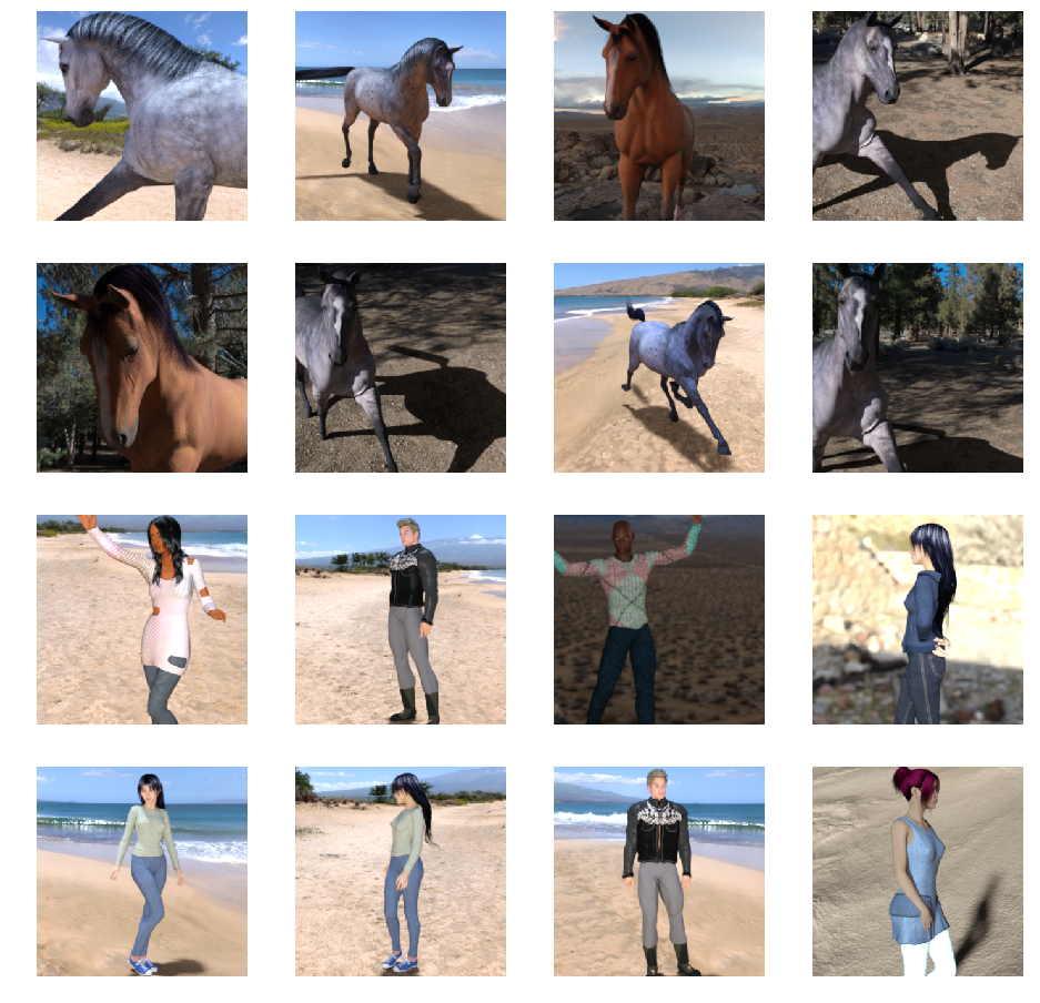
ここで、8 枚の馬の写真と 8 枚の人間の写真を表示します。セルの再実行で毎回新しいバッチを表示できます。
# Set up matplotlib fig, and size it to fit 4x4 pics
fig = plt.gcf()
fig.set_size_inches(ncols * 4, nrows * 4)

pic_index += 8
next_horse_pix = [os.path.join(train_horse_dir, fname)
                for fname in train_horse_names[pic_index-8:pic_index]]
next_human_pix = [os.path.join(train_human_dir, fname)
                for fname in train_human_names[pic_index-8:pic_index]]

for i, img_path in enumerate(next_horse_pix+next_human_pix):
  # Set up subplot; subplot indices start at 1
  sp = plt.subplot(nrows, ncols, i + 1)
  sp.axis('Off') # Don't show axes (or gridlines)

  img = mpimg.imread(img_path)
  plt.imshow(img)

plt.show()
以下に、馬と人間のさまざまなポーズや向きの画像を表示します。
5. モデルを定義する
モデルの定義を開始する。
まず、次のように TensorFlow をインポートします。
import tensorflow as tf
次に、畳み込みレイヤを追加して最終結果をフラット化し、密結合したレイヤにフィードします。最後に、密結合したレイヤを追加します。
なお、2 クラス分類の問題(バイナリ分類問題)に直面しているため、ネットワークは Sigmoid アクティベーションにより終了し、ネットワークの出力は 0 ~ 1 のスカラーになり、現在の画像がクラス 1 になる確率がエンコードされます(クラス 0 ではありません)。
model = tf.keras.models.Sequential([
    # Note the input shape is the desired size of the image 300x300 with 3 bytes color
    # This is the first convolution
    tf.keras.layers.Conv2D(16, (3,3), activation='relu', input_shape=(300, 300, 3)),
    tf.keras.layers.MaxPooling2D(2, 2),
    # The second convolution
    tf.keras.layers.Conv2D(32, (3,3), activation='relu'),
    tf.keras.layers.MaxPooling2D(2,2),
    # The third convolution
    tf.keras.layers.Conv2D(64, (3,3), activation='relu'),
    tf.keras.layers.MaxPooling2D(2,2),
    # The fourth convolution
    tf.keras.layers.Conv2D(64, (3,3), activation='relu'),
    tf.keras.layers.MaxPooling2D(2,2),
    # The fifth convolution
    tf.keras.layers.Conv2D(64, (3,3), activation='relu'),
    tf.keras.layers.MaxPooling2D(2,2),
    # Flatten the results to feed into a DNN
    tf.keras.layers.Flatten(),
    # 512 neuron hidden layer
    tf.keras.layers.Dense(512, activation='relu'),
    # Only 1 output neuron. It will contain a value from 0-1 where 0 for 1 class ('horses') and 1 for the other ('humans')
    tf.keras.layers.Dense(1, activation='sigmoid')
])
model.summary() メソッド呼び出しは、ネットワークの概要を出力します。
model.summary()
結果はこちらでご確認いただけます。
Layer (type)                 Output Shape              Param #
=================================================================
conv2d (Conv2D)              (None, 298, 298, 16)      448
_________________________________________________________________
max_pooling2d (MaxPooling2D) (None, 149, 149, 16)      0
_________________________________________________________________
conv2d_1 (Conv2D)            (None, 147, 147, 32)      4640
_________________________________________________________________
max_pooling2d_1 (MaxPooling2 (None, 73, 73, 32)        0
_________________________________________________________________
conv2d_2 (Conv2D)            (None, 71, 71, 64)        18496
_________________________________________________________________
max_pooling2d_2 (MaxPooling2 (None, 35, 35, 64)        0
_________________________________________________________________
conv2d_3 (Conv2D)            (None, 33, 33, 64)        36928
_________________________________________________________________
max_pooling2d_3 (MaxPooling2 (None, 16, 16, 64)        0
_________________________________________________________________
conv2d_4 (Conv2D)            (None, 14, 14, 64)        36928
_________________________________________________________________
max_pooling2d_4 (MaxPooling2 (None, 7, 7, 64)          0
_________________________________________________________________
flatten (Flatten)            (None, 3136)              0
_________________________________________________________________
dense (Dense)                (None, 512)               1606144
_________________________________________________________________
dense_1 (Dense)              (None, 1)                 513
=================================================================
Total params: 1,704,097
Trainable params: 1,704,097
Non-trainable params: 0
出力シェイプの列には、連続する各レイヤで特徴マップのサイズがどのように変化するかが表示されます。畳み込み層は、パディングにより対象物マップのサイズを少し小さくし、各プールレイヤは寸法を半分にします。
6. モデルをコンパイルする
次に、モデル トレーニングの仕様を構成します。バイナリ分類の問題であり、最後のアクティベーションはシグモイドであるため、binary_crossentropy 損失でモデルをトレーニングします。(損失指標の詳細については、ML の降順をご覧ください)。rmsprop オプティマイザーを学習率 0.001 で使用します。トレーニング中に分類の精度をモニタリングします。
from tensorflow.keras.optimizers import RMSprop

model.compile(loss='binary_crossentropy',
              optimizer=RMSprop(lr=0.001),
              metrics=['acc'])
7. 生成ツールからモデルをトレーニングする
ソース フォルダ内の写真を読み取り、float32 テンソルに変換して(ラベルを付けて)ネットワークにフィードするデータ生成ツールを設定します。
トレーニング画像用と検証画像用の生成ツールが 1 つずつあります。生成ツールを使用すると、300x300 のサイズの画像とそのラベル(バイナリ)が生成されます。
すでにご存じかもしれませんが、ニューラル ネットワークに送信されるデータは、ネットワークによる処理の影響を受けやすくなるよう、なんらかの方法で正規化する必要があります。(CNN に未加工のピクセルをフィードすることは珍しくありません)。この場合、ピクセル値を [0, 1] の範囲内に正規化して画像を前処理します(元々はすべての値が [0, 255] の範囲内に収まります)。
Keras では、keras.preprocessing.image.ImageDataGenerator クラスを介して rescale パラメータを使用します。その ImageDataGenerator クラスを使用すると、.flow(データ、ラベル)または .flow_from_directory(ディレクトリ)を介して拡張画像バッチ(およびそのラベル)のジェネレータをインスタンス化できます。これらの生成ツールは、データ ジェネレータを入力として受け入れる Keras モデルメソッド(fit_generator、evaluate_generator、predict_generator)で使用できます。
from tensorflow.keras.preprocessing.image import ImageDataGenerator

# All images will be rescaled by 1./255
train_datagen = ImageDataGenerator(rescale=1./255)

# Flow training images in batches of 128 using train_datagen generator
train_generator = train_datagen.flow_from_directory(
        '/tmp/horse-or-human/',  # This is the source directory for training images
        target_size=(300, 300),  # All images will be resized to 150x150
        batch_size=128,
        # Since we use binary_crossentropy loss, we need binary labels
        class_mode='binary')
8. トレーニングを実施する
15 エポックのトレーニングを行います。(実行には数分かかることがあります)。
history = model.fit(
      train_generator,
      steps_per_epoch=8,
      epochs=15,
      verbose=1)
エポックごとの値を確認します。
[損失] と [精度] は、トレーニングの進捗状況を示す優れた指標です。トレーニング データの分類について推測し、既知のラベルに対して測定して、結果を計算します。正確性は推測の正確さの一部です。
Epoch 1/15
9/9 [==============================] - 9s 1s/step - loss: 0.8662 - acc: 0.5151
Epoch 2/15
9/9 [==============================] - 8s 927ms/step - loss: 0.7212 - acc: 0.5969
Epoch 3/15
9/9 [==============================] - 8s 921ms/step - loss: 0.6612 - acc: 0.6592
Epoch 4/15
9/9 [==============================] - 8s 925ms/step - loss: 0.3135 - acc: 0.8481
Epoch 5/15
9/9 [==============================] - 8s 919ms/step - loss: 0.4640 - acc: 0.8530
Epoch 6/15
9/9 [==============================] - 8s 896ms/step - loss: 0.2306 - acc: 0.9231
Epoch 7/15
9/9 [==============================] - 8s 915ms/step - loss: 0.1464 - acc: 0.9396
Epoch 8/15
9/9 [==============================] - 8s 935ms/step - loss: 0.2663 - acc: 0.8919
Epoch 9/15
9/9 [==============================] - 8s 883ms/step - loss: 0.0772 - acc: 0.9698
Epoch 10/15
9/9 [==============================] - 9s 951ms/step - loss: 0.0403 - acc: 0.9805
Epoch 11/15
9/9 [==============================] - 8s 891ms/step - loss: 0.2618 - acc: 0.9075
Epoch 12/15
9/9 [==============================] - 8s 902ms/step - loss: 0.0434 - acc: 0.9873
Epoch 13/15
9/9 [==============================] - 8s 904ms/step - loss: 0.0187 - acc: 0.9932
Epoch 14/15
9/9 [==============================] - 9s 951ms/step - loss: 0.0974 - acc: 0.9649
Epoch 15/15
9/9 [==============================] - 8s 877ms/step - loss: 0.2859 - acc: 0.9338
9. モデルをテストする
次に、モデルを使用して予測を実行します。コードを使用すると、ファイル システムから 1 つ以上のファイルを選択できます。次に、それらをアップロードしてモデルで実行することで、オブジェクトが馬であるか人間であるかが示されます。
インターネットからファイル システムに画像をダウンロードして、ぜひお試しください。トレーニングの精度が 99% を超えるにもかかわらず、ネットワークで多くの間違いが生じる場合があります。
これは、過学習と呼ばれるもので、つまりニューラル ネットワークが極めて限られたデータでトレーニングされるということです(各クラスの画像は約 500 枚です)。そのため、トレーニング セットに含まれる画像とよく似た画像を認識するのに優れていますが、トレーニング セットにない画像では失敗する可能性があります。
つまり、トレーニングするデータが多いほど、最終的なネットワークの改善につながることを証明できるデータポイントです。
画像を拡張するなど、データが限られているにもかかわらずトレーニングを改善するためにさまざまな手法を使用できますが、この Codelab では扱いません。
import numpy as np
from google.colab import files
from keras.preprocessing import image

uploaded = files.upload()

for fn in uploaded.keys():

  # predicting images
  path = '/content/' + fn
  img = image.load_img(path, target_size=(300, 300))
  x = image.img_to_array(img)
  x = np.expand_dims(x, axis=0)

  images = np.vstack([x])
  classes = model.predict(images, batch_size=10)
  print(classes[0])
  if classes[0]>0.5:
    print(fn + " is a human")
  else:
    print(fn + " is a horse")
たとえば、次の画像を使用してテストしたいとします。

この COLA が生成するデータは以下のとおりです。
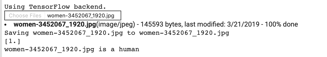
マンガのグラフィックであるにもかかわらず、引き続き正しく分類されています。
次の画像も適切に分類されています。
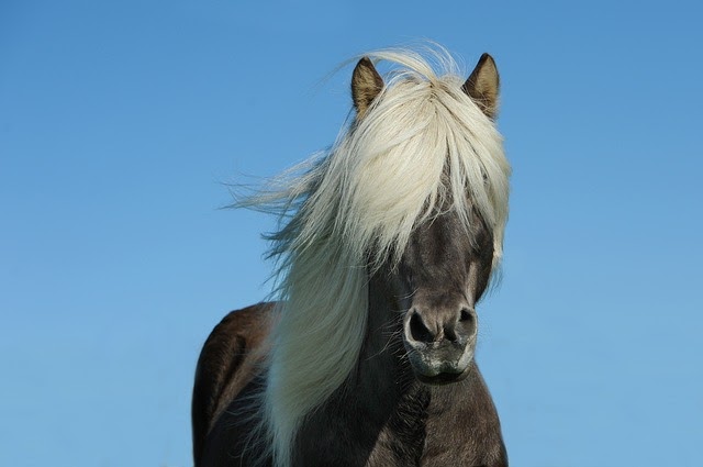
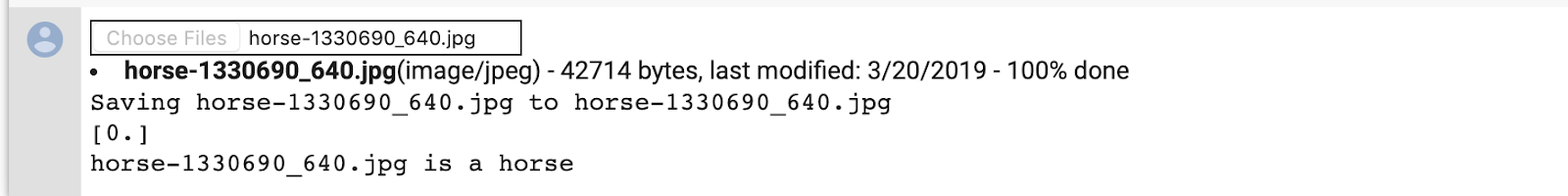
お持ちの画像で試してみましょう。
10. 中間表現の可視化
CNN が学習した特徴を把握するために、CNN を通過する入力の変換を可視化するのがおすすめです。
トレーニング セットから画像をランダムに選択し、各行がレイヤの出力で、行内の各画像がその出力特徴マップの特定のフィルタになる図を生成します。このセルを再実行して、さまざまなトレーニング画像の中間表現を生成します。
import numpy as np
import random
from tensorflow.keras.preprocessing.image import img_to_array, load_img

# Let's define a new Model that will take an image as input, and will output
# intermediate representations for all layers in the previous model after
# the first.
successive_outputs = [layer.output for layer in model.layers[1:]]
#visualization_model = Model(img_input, successive_outputs)
visualization_model = tf.keras.models.Model(inputs = model.input, outputs = successive_outputs)
# Let's prepare a random input image from the training set.
horse_img_files = [os.path.join(train_horse_dir, f) for f in train_horse_names]
human_img_files = [os.path.join(train_human_dir, f) for f in train_human_names]
img_path = random.choice(horse_img_files + human_img_files)

img = load_img(img_path, target_size=(300, 300))  # this is a PIL image
x = img_to_array(img)  # Numpy array with shape (150, 150, 3)
x = x.reshape((1,) + x.shape)  # Numpy array with shape (1, 150, 150, 3)

# Rescale by 1/255
x /= 255

# Let's run our image through our network, thus obtaining all
# intermediate representations for this image.
successive_feature_maps = visualization_model.predict(x)

# These are the names of the layers, so can have them as part of our plot
layer_names = [layer.name for layer in model.layers]

# Now let's display our representations
for layer_name, feature_map in zip(layer_names, successive_feature_maps):
  if len(feature_map.shape) == 4:
    # Just do this for the conv / maxpool layers, not the fully-connected layers
    n_features = feature_map.shape[-1]  # number of features in feature map
    # The feature map has shape (1, size, size, n_features)
    size = feature_map.shape[1]
    # We will tile our images in this matrix
    display_grid = np.zeros((size, size * n_features))
    for i in range(n_features):
      # Postprocess the feature to make it visually palatable
      x = feature_map[0, :, :, i]
      x -= x.mean()
      if x.std()>0:
        x /= x.std()
      x *= 64
      x += 128
      x = np.clip(x, 0, 255).astype('uint8')
      # We'll tile each filter into this big horizontal grid
      display_grid[:, i * size : (i + 1) * size] = x
    # Display the grid
    scale = 20. / n_features
    plt.figure(figsize=(scale * n_features, scale))
    plt.title(layer_name)
    plt.grid(False)
    plt.imshow(display_grid, aspect='auto', cmap='viridis')
結果の例を次に示します。
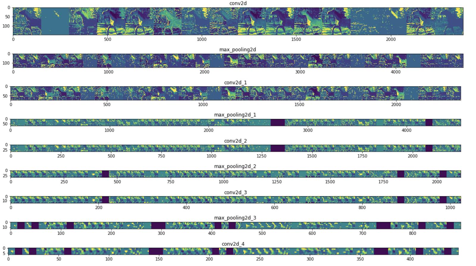
ご覧のとおり、画像の未加工のピクセルから、抽象的かつコンパクトな表現へと移行しています。ダウンストリームでは、ネットワークが何に注意を払うのかが浮き彫りになり、有効化される機能が減少していきます。ほとんどは 0 に設定されます。これをスパース性といいます。表現のスパース性はディープ ラーニングの重要な特長です。
これらの表現は、画像の元のピクセルに関する情報はますます少なくなり、画像のクラスについての情報はますます洗練されています。CNN(一般的にはディープ ネットワーク)は、情報抽出パイプラインと考えることができます。
11. 完了
CNN を使用して複雑な画像を補正する方法を学習しました。コンピュータ ビジョン モデルをさらに強化する方法については、大規模なデータセットで畳み込みニューラル ネットワーク(CNN)を使用するをご覧ください。