इस पेज का अनुवाद Cloud Translation API से किया गया है.

कॉम्प्लेक्स इमेज के साथ कन्वर्ज़न न्यूरल नेटवर्क (CNN) का इस्तेमाल करना

1. शुरू करने से पहले

इस कोडलैब में आप घोड़ों का इस्तेमाल करेंगे, ताकि घोड़ों और इंसानों की इमेज की कैटगरी तय की जा सके. आप इस लैब में TensorFlow का इस्तेमाल करके, ऐसा CNN बना सकते हैं जिसे घोड़ों और इंसानों की इमेज पहचानने और उन्हें अलग-अलग कैटगरी में बांटने की ट्रेनिंग दी गई हो.

ज़रूरी शर्तें

अगर आपने पहले TensorFlow का इस्तेमाल करके कन्वर्ज़न नहीं बनाए हैं, तो हो सकता है कि आप कंवोलेशन बनाना और पूल करना कोडलैब (कोड बनाना सीखना) पूरा करना चाहें. इसके लिए, हम कन्वोल्यूशन और पूलिंग की सुविधा देते हैं और कंप्यूटर विज़न को बेहतर बनाने के लिए कन्वोल्यूशन न्यूरल नेटवर्क (CNN) बनाते हैं, जहां हम इमेज की पहचान करने के लिए कंप्यूटर को ज़्यादा बेहतर बनाने का तरीका बताएंगे.

आप क्या #39;जानेंगे

इमेज में दिख रही सुविधाओं की पहचान करने के लिए, कंप्यूटर को ट्रेनिंग देने का तरीका

आप क्या बनाते हैं

एक मधुर न्यूरल नेटवर्क, जो घोड़ों की तस्वीरों और इंसानों की तस्वीरों के बीच अंतर कर सकता है

आपको क्या चाहिए

आप Colab में चल रहे कोडलैब के बाकी कोड के लिए कोड देख सकते हैं.

आपको #39; TensorFlow इंस्टॉल करने के साथ ही, पिछले कोडलैब में इंस्टॉल की गई लाइब्रेरी की भी ज़रूरत होगी.

2. शुरू करना: डेटा पाना

ऐसा करने के लिए एक घोड़ा या ह्यूमैनस क्लासिफ़ायर बनाकर, आप ऐसा कर सकते हैं. इस टूल की मदद से आप बता पाएंगे कि इमेज में कोई घोड़ा या इंसान मौजूद है या नहीं. नेटवर्क में उन सुविधाओं को पहचानने के लिए प्रशिक्षित है जिनमें से यह तय किया जाता है कि कौनसी इमेज कैसी है. इससे पहले कि आप ट्रेनिंग कर सकें, आपको डेटा की कुछ प्रोसेसिंग करनी होगी.

सबसे पहले, डेटा डाउनलोड करें:

!wget --no-check-certificate https://storage.googleapis.com/laurencemoroney-blog.appspot.com/horse-or-human.zip  -O /tmp/horse-or-human.zip

नीचे दिया गया Python कोड, ऑपरेटिंग सिस्टम लाइब्रेरी का इस्तेमाल करने के लिए, ओएस लाइब्रेरी का इस्तेमाल करेगा. इससे, आपको फ़ाइल सिस्टम और ज़िप फ़ाइल लाइब्रेरी का ऐक्सेस मिल जाएगा. इससे आपको डेटा अनज़िप करने में मदद मिलेगी.

import os
import zipfile
 
local_zip = '/tmp/horse-or-human.zip'
zip_ref = zipfile.ZipFile(local_zip, 'r')
zip_ref.extractall('/tmp/horse-or-human')
zip_ref.close()

ज़िप फ़ाइल के कॉन्टेंट को बेस डायरेक्ट्री /tmp/horse-or-human में निकाला जाता है, जिसमें घोड़े और मैन्युअल सबडायरेक्ट्री होती हैं.

कम शब्दों में कहें, तो यह ट्रेनिंग डेटा वह होता है जिसका इस्तेमाल न्यूरल नेटवर्क मॉडल को यह बताने के लिए किया जाता है कि "घोड़ा कैसा दिखता है; & "यह कैसा इंसान होता है.&कोटेशन;

3. डेटा को लेबल करने और तैयार करने के लिए, ImageGenator का इस्तेमाल करें

आप साफ़ तौर पर इमेज को घोड़े या इंसान के तौर पर लेबल नहीं करते.

बाद में आपको #39;ImageDataGenerator का इस्तेमाल होता हुआ कुछ दिखेगा. यह सबडायरेक्ट्री से इमेज पढ़ता है और उन्हें उस सबडायरेक्ट्री के नाम से अपने-आप लेबल कर देता है. उदाहरण के लिए, आपके पास ट्रेनिंग डायरेक्ट्री है जिसमें घोड़ों की डायरेक्ट्री और इंसान की डायरेक्ट्री शामिल है. ImageDataGenerator कोडिंग के चरण को कम करते हुए, आपके लिए इमेज को सही तरीके से लेबल करेगा.

उनमें से हर डायरेक्ट्री के बारे में बताएं.

# Directory with our training horse pictures
train_horse_dir = os.path.join('/tmp/horse-or-human/horses')
 
# Directory with our training human pictures
train_human_dir = os.path.join('/tmp/horse-or-human/humans')

अब, देखें कि फ़ाइल के नाम घोड़ों और लोगों की ट्रेनिंग डायरेक्ट्री में कैसे दिखते हैं:

train_horse_names = os.listdir(train_horse_dir)
print(train_horse_names[:10])
train_human_names = os.listdir(train_human_dir)
print(train_human_names[:10])

डायरेक्ट्री में घोड़े और मानव इमेज की कुल संख्या देखें:

print('total training horse images:', len(os.listdir(train_horse_dir)))
print('total training human images:', len(os.listdir(train_human_dir)))

4. डेटा को एक्सप्लोर करें

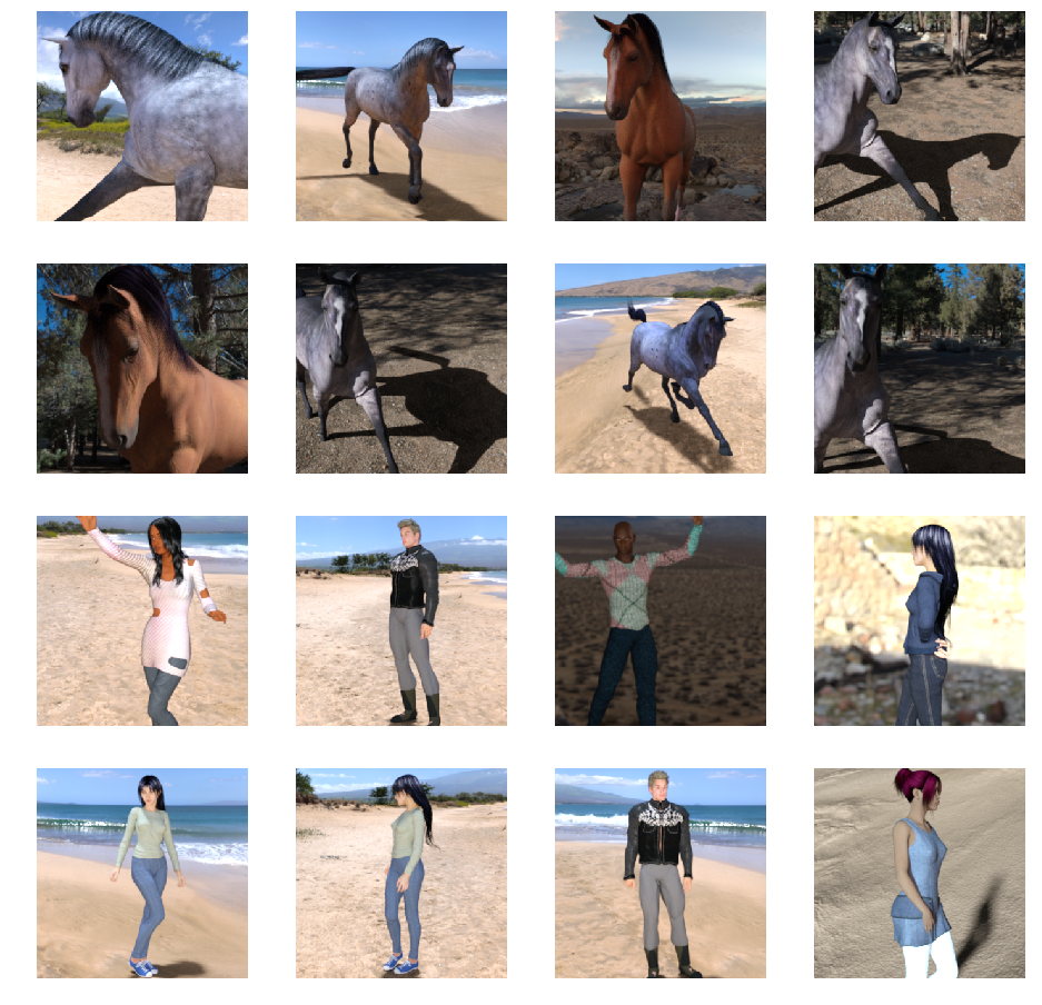
कुछ तस्वीरों पर एक नज़र डालकर उन्हें बेहतर तरीके से समझें.

सबसे पहले, matplot पैरामीटर कॉन्फ़िगर करें:

%matplotlib inline
 
import matplotlib.pyplot as plt
import matplotlib.image as mpimg
 
# Parameters for our graph; we'll output images in a 4x4 configuration
nrows = 4
ncols = 4
 
# Index for iterating over images
pic_index = 0

अब, घोड़े की आठ तस्वीरों और आठ इंसान की तस्वीरों का बैच दिखाएं. हर बार नया बैच देखने के लिए, सेल को फिर से चलाया जा सकता है.

# Set up matplotlib fig, and size it to fit 4x4 pics
fig = plt.gcf()
fig.set_size_inches(ncols * 4, nrows * 4)
 
pic_index += 8
next_horse_pix = [os.path.join(train_horse_dir, fname) 
                for fname in train_horse_names[pic_index-8:pic_index]]
next_human_pix = [os.path.join(train_human_dir, fname) 
                for fname in train_human_names[pic_index-8:pic_index]]
 
for i, img_path in enumerate(next_horse_pix+next_human_pix):
  # Set up subplot; subplot indices start at 1
  sp = plt.subplot(nrows, ncols, i + 1)
  sp.axis('Off') # Don't show axes (or gridlines)
 
  img = mpimg.imread(img_path)
  plt.imshow(img)
 
plt.show()

यहां अलग-अलग मुद्राओं और ओरिएंटेशन में घोड़ों और इंसानों को दिखाने वाली इमेज दी गई हैं:

5. मॉडल तय करें

मॉडल तय करना शुरू करें.

TensorFlow इंपोर्ट करके शुरू करें:

import tensorflow as tf

फिर, घुटनों के अंदर लेयर जोड़ें और आखिरी नतीजे को घनी कनेक्ट की गई लेयर में फ़ीड करने के लिए फ़्लैट करें. आखिर में, घनी आबादी वाले लेयर जोड़ें.

ध्यान दें कि आपकी 'दो-क्लास की क्लासिफ़िकेशन से जुड़ी समस्या (बाइनरी क्लासिफ़िकेशन की समस्या) का सामना कर रहा है और आप#39 ऐक्टिवेशन के साथ खत्म हो जाएंगे, ताकि आपके नेटवर्क के आउटपुट में 0 और 1 के बीच का एक स्केलर हो सके (इसका मतलब है कि मौजूदा इमेज क्लास 1 है).

model = tf.keras.models.Sequential([
    # Note the input shape is the desired size of the image 300x300 with 3 bytes color
    # This is the first convolution
    tf.keras.layers.Conv2D(16, (3,3), activation='relu', input_shape=(300, 300, 3)),
    tf.keras.layers.MaxPooling2D(2, 2),
    # The second convolution
    tf.keras.layers.Conv2D(32, (3,3), activation='relu'),
    tf.keras.layers.MaxPooling2D(2,2),
    # The third convolution
    tf.keras.layers.Conv2D(64, (3,3), activation='relu'),
    tf.keras.layers.MaxPooling2D(2,2),
    # The fourth convolution
    tf.keras.layers.Conv2D(64, (3,3), activation='relu'),
    tf.keras.layers.MaxPooling2D(2,2),
    # The fifth convolution
    tf.keras.layers.Conv2D(64, (3,3), activation='relu'),
    tf.keras.layers.MaxPooling2D(2,2),
    # Flatten the results to feed into a DNN
    tf.keras.layers.Flatten(),
    # 512 neuron hidden layer
    tf.keras.layers.Dense(512, activation='relu'),
    # Only 1 output neuron. It will contain a value from 0-1 where 0 for 1 class ('horses') and 1 for the other ('humans')
    tf.keras.layers.Dense(1, activation='sigmoid')
])

model.summary() तरीके का कॉल, नेटवर्क की खास जानकारी प्रिंट करता है.

model.summary()

आप नतीजों को यहां देख सकते हैं:

Layer (type)                 Output Shape              Param #   
=================================================================
conv2d (Conv2D)              (None, 298, 298, 16)      448       
_________________________________________________________________
max_pooling2d (MaxPooling2D) (None, 149, 149, 16)      0         
_________________________________________________________________
conv2d_1 (Conv2D)            (None, 147, 147, 32)      4640      
_________________________________________________________________
max_pooling2d_1 (MaxPooling2 (None, 73, 73, 32)        0         
_________________________________________________________________
conv2d_2 (Conv2D)            (None, 71, 71, 64)        18496     
_________________________________________________________________
max_pooling2d_2 (MaxPooling2 (None, 35, 35, 64)        0         
_________________________________________________________________
conv2d_3 (Conv2D)            (None, 33, 33, 64)        36928     
_________________________________________________________________
max_pooling2d_3 (MaxPooling2 (None, 16, 16, 64)        0         
_________________________________________________________________
conv2d_4 (Conv2D)            (None, 14, 14, 64)        36928     
_________________________________________________________________
max_pooling2d_4 (MaxPooling2 (None, 7, 7, 64)          0         
_________________________________________________________________
flatten (Flatten)            (None, 3136)              0         
_________________________________________________________________
dense (Dense)                (None, 512)               1606144   
_________________________________________________________________
dense_1 (Dense)              (None, 1)                 513       
=================================================================
Total params: 1,704,097
Trainable params: 1,704,097
Non-trainable params: 0

आउटपुट आकार के कॉलम से पता चलता है कि हर एक लेयर में, आपके फ़ीचर मैप का साइज़ कैसे बदलता है. कॉन्वोल्यूशन लेयर, पैडिंग की वजह से सुविधा मैप के साइज़ को थोड़ा कम कर देती हैं और हर पूलिंग डाइमेंशन को आधा कर देती है.

6. मॉडल को कंपाइल करें

इसके बाद, मॉडल प्रशिक्षण के लिए विवरण कॉन्फ़िगर करें. अपने मॉडल को binary_crossentropy हानि के साथ प्रशिक्षित करें क्योंकि यह बाइनरी वर्गीकरण की समस्या और आपका अंतिम सक्रियण एक साइज़ है. (ऐप्लिकेशन के नुकसान की मेट्रिक के बारे में फिर से जानने के लिए, एमएल को घटते क्रम में लगाएं देखें.) rmsprop ऑप्टिमाइज़र का इस्तेमाल करके, 0.001 के लर्निंग रेट का इस्तेमाल करें. ट्रेनिंग के दौरान, श्रेणियों के सटीक होने की निगरानी करें.

from tensorflow.keras.optimizers import RMSprop
 
model.compile(loss='binary_crossentropy',
              optimizer=RMSprop(lr=0.001),
              metrics=['acc'])

7. मॉडल से जनरेटर जनरेट करें

डेटा जनरेटर को सेट अप करें, जो आपके सोर्स फ़ोल्डर में मौजूद तस्वीरों को पढ़ते हैं, उन्हें फ़्लोटर 22 में बदलें और उन्हें अपने नेटवर्क में फ़ीड करें.

आपकी ट्रेनिंग इमेज के लिए एक जनरेटर और पुष्टि करने वाली इमेज के लिए एक जनरेटर होगा. आपके जनरेटर से 300x300 साइज़ और उनकी लेबल (बाइनरी) की इमेज मिलेंगी.

जैसा कि आपको पहले से पता होगा कि न्यूरल नेटवर्क में जाने वाले डेटा को आम तौर पर किसी सामान्य तरीके से सामान्य बनाया जाना चाहिए, ताकि नेटवर्क उसे प्रोसेस कर सके. (CNAME की मदद से किसी रॉ पिक्सल को CNN में फ़ीड करना आम बात नहीं है.) आपके मामले में, पिक्सल वैल्यू को 0, 1] की रेंज में सामान्य करके, अपनी इमेज को पहले से प्रोसेस किया जाता है (मूल रूप से सभी वैल्यू [0, 255] रेंज में होती हैं).

Keras में, रीस्केल पैरामीटर का इस्तेमाल करके, keras.preprocessing.image.ImageDataGenerator क्लास से किया जा सकता है. ImageDataGenerator क्लास की मदद से, आप .flow (डेटा, लेबल) या .flow_from_directory(डायरेक्ट्री) का इस्तेमाल करके ऑगमेंटेड इमेज बैच(और उनके लेबल) के जनरेटर को इंस्टैंशिएट करें. इसके बाद, जनरेटर का इस्तेमाल, Keras मॉडल के उन तरीकों के साथ किया जा सकता है जो इनपुट के तौर पर डेटा जनरेटर को स्वीकार करते हैं: fit_generator, evaluate_generator, और predict_generator.

from tensorflow.keras.preprocessing.image import ImageDataGenerator
 
# All images will be rescaled by 1./255
train_datagen = ImageDataGenerator(rescale=1./255)
 
# Flow training images in batches of 128 using train_datagen generator
train_generator = train_datagen.flow_from_directory(
        '/tmp/horse-or-human/',  # This is the source directory for training images
        target_size=(300, 300),  # All images will be resized to 150x150
        batch_size=128,
        # Since we use binary_crossentropy loss, we need binary labels
        class_mode='binary')

8. ट्रेनिंग लें

15 युगों के लिए ट्रेन (इसे चलाने में कुछ मिनट लग सकते हैं.)

history = model.fit(
      train_generator,
      steps_per_epoch=8,  
      epochs=15,
      verbose=1)

हर epoch में वैल्यू देखें.

घाटी और सटीक काम करना, ट्रेनिंग की प्रगति का एक बेहतरीन संकेत है. यह ट्रेनिंग डेटा को अलग-अलग कैटगरी में बांटने और अनुमान वाले लेबल की मदद से इसका आकलन करने में मदद करता है. सही अनुमानों का हिस्सा 'सही' है.

Epoch 1/15
9/9 [==============================] - 9s 1s/step - loss: 0.8662 - acc: 0.5151
Epoch 2/15
9/9 [==============================] - 8s 927ms/step - loss: 0.7212 - acc: 0.5969
Epoch 3/15
9/9 [==============================] - 8s 921ms/step - loss: 0.6612 - acc: 0.6592
Epoch 4/15
9/9 [==============================] - 8s 925ms/step - loss: 0.3135 - acc: 0.8481
Epoch 5/15
9/9 [==============================] - 8s 919ms/step - loss: 0.4640 - acc: 0.8530
Epoch 6/15
9/9 [==============================] - 8s 896ms/step - loss: 0.2306 - acc: 0.9231
Epoch 7/15
9/9 [==============================] - 8s 915ms/step - loss: 0.1464 - acc: 0.9396
Epoch 8/15
9/9 [==============================] - 8s 935ms/step - loss: 0.2663 - acc: 0.8919
Epoch 9/15
9/9 [==============================] - 8s 883ms/step - loss: 0.0772 - acc: 0.9698
Epoch 10/15
9/9 [==============================] - 9s 951ms/step - loss: 0.0403 - acc: 0.9805
Epoch 11/15
9/9 [==============================] - 8s 891ms/step - loss: 0.2618 - acc: 0.9075
Epoch 12/15
9/9 [==============================] - 8s 902ms/step - loss: 0.0434 - acc: 0.9873
Epoch 13/15
9/9 [==============================] - 8s 904ms/step - loss: 0.0187 - acc: 0.9932
Epoch 14/15
9/9 [==============================] - 9s 951ms/step - loss: 0.0974 - acc: 0.9649
Epoch 15/15
9/9 [==============================] - 8s 877ms/step - loss: 0.2859 - acc: 0.9338

9. मॉडल की जांच करें

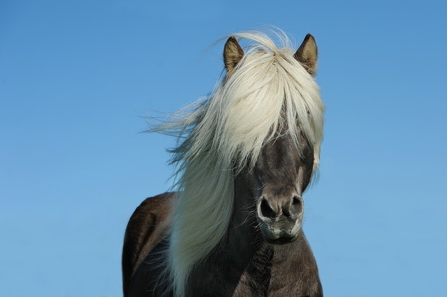
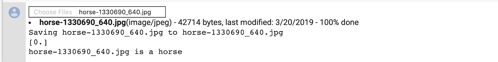
अब मॉडल का इस्तेमाल करके अनुमान लगाएं. कोड आपको अपने फ़ाइल सिस्टम से एक या ज़्यादा फ़ाइलें चुनने देगा. फिर यह उन्हें अपलोड करेगा और मॉडल के हिसाब से चलाएगा. इससे यह पता चलेगा कि ऑब्जेक्ट घोड़ा है या इंसान.

आप इंटरनेट से इमेज डाउनलोड करके उन्हें अपने फ़ाइल सिस्टम में डाउनलोड कर सकते हैं! ध्यान दें कि आपने देखा कि नेटवर्क 99% से ज़्यादा सही होने के बावजूद, कई गलतियां करता है.

यह इसलिए होता है, क्योंकिओवरफ़िटिंग का मतलब है कि न्यूरल नेटवर्क बहुत सीमित डेटा से ट्रेनिंग लेता है. हर क्लास की सिर्फ़ 500 इमेज ही तैयार की जा सकती हैं. इसलिए, यह उन इमेज की पहचान करना बहुत अच्छा होता है जो ट्रेनिंग सेट में मौजूद इमेज की तरह दिखती हैं. हालांकि, ये उन इमेज को पहचानने में बहुत असफल हो सकती हैं जो ट्रेनिंग सेट में मौजूद नहीं होती हैं.

यह एक डेटापॉइंट है जो यह साबित करता है कि आप जितने ज़्यादा डेटा को चालू करेंगे उतना ही आपका फ़ाइनल नेटवर्क बेहतर होगा!

ऐसी कई तकनीकें हैं जिनका इस्तेमाल आपकी ट्रेनिंग को बेहतर बनाने के लिए किया जा सकता है. हालांकि, इसमें डेटा की बढ़ोतरी के बारे में सीमित जानकारी होने के बावजूद ऐसा किया जा सकता है. हालांकि, इसमें कई ऐसी चीज़ें हैं जो इस कोडलैब के दायरे से बाहर हैं.

import numpy as np
from google.colab import files
from keras.preprocessing import image
 
uploaded = files.upload()
 
for fn in uploaded.keys():
 
  # predicting images
  path = '/content/' + fn
  img = image.load_img(path, target_size=(300, 300))
  x = image.img_to_array(img)
  x = np.expand_dims(x, axis=0)
 
  images = np.vstack([x])
  classes = model.predict(images, batch_size=10)
  print(classes[0])
  if classes[0]>0.5:
    print(fn + " is a human")
  else:
    print(fn + " is a horse")

उदाहरण के लिए, मान लें कि आप इस इमेज से जांच करना चाहते हैं:

यहां दिया गया है कि कोलैब क्या बनाता है:

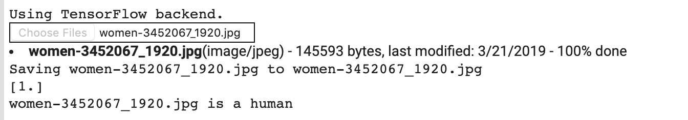
भले ही, यह कार्टून ग्राफ़िक हो, लेकिन इसकी कैटगरी सही तरीके से तय की जाती है.

नीचे दी गई इमेज सही कैटगरी में भी दिखती है:

अपनी खुद की कुछ इमेज आज़माकर देखें!

10. बीच के प्रतिनिधित्व को विज़ुअलाइज़ करें

सीएनएन ने जो कुछ भी सीखा है उसके बारे में जानने के लिए, एक मज़ेदार तरीका यह है कि आप सीएनएन में जाकर, इनपुट में बदलाव कैसे करें.

ट्रेनिंग सेट से किसी भी इमेज को चुनें, फिर एक ऐसी इमेज जनरेट करें जिसमें हर लाइन किसी लेयर का आउटपुट हो और उस लाइन में मौजूद हर इमेज, उस आउटपुट फ़ीचर मैप में एक खास फ़िल्टर हो. अलग-अलग तरह की ट्रेनिंग इमेज के लिए, बीच के प्रतिनिधि बनाने के लिए उस सेल को फिर से चलाएं.

import numpy as np
import random
from tensorflow.keras.preprocessing.image import img_to_array, load_img
 
# Let's define a new Model that will take an image as input, and will output
# intermediate representations for all layers in the previous model after
# the first.
successive_outputs = [layer.output for layer in model.layers[1:]]
#visualization_model = Model(img_input, successive_outputs)
visualization_model = tf.keras.models.Model(inputs = model.input, outputs = successive_outputs)
# Let's prepare a random input image from the training set.
horse_img_files = [os.path.join(train_horse_dir, f) for f in train_horse_names]
human_img_files = [os.path.join(train_human_dir, f) for f in train_human_names]
img_path = random.choice(horse_img_files + human_img_files)
 
img = load_img(img_path, target_size=(300, 300))  # this is a PIL image
x = img_to_array(img)  # Numpy array with shape (150, 150, 3)
x = x.reshape((1,) + x.shape)  # Numpy array with shape (1, 150, 150, 3)
 
# Rescale by 1/255
x /= 255
 
# Let's run our image through our network, thus obtaining all
# intermediate representations for this image.
successive_feature_maps = visualization_model.predict(x)
 
# These are the names of the layers, so can have them as part of our plot
layer_names = [layer.name for layer in model.layers]
 
# Now let's display our representations
for layer_name, feature_map in zip(layer_names, successive_feature_maps):
  if len(feature_map.shape) == 4:
    # Just do this for the conv / maxpool layers, not the fully-connected layers
    n_features = feature_map.shape[-1]  # number of features in feature map
    # The feature map has shape (1, size, size, n_features)
    size = feature_map.shape[1]
    # We will tile our images in this matrix
    display_grid = np.zeros((size, size * n_features))
    for i in range(n_features):
      # Postprocess the feature to make it visually palatable
      x = feature_map[0, :, :, i]
      x -= x.mean()
      if x.std()>0:
        x /= x.std()
      x *= 64
      x += 128
      x = np.clip(x, 0, 255).astype('uint8')
      # We'll tile each filter into this big horizontal grid
      display_grid[:, i * size : (i + 1) * size] = x
    # Display the grid
    scale = 20. / n_features
    plt.figure(figsize=(scale * n_features, scale))
    plt.title(layer_name)
    plt.grid(False)
    plt.imshow(display_grid, aspect='auto', cmap='viridis')

यहां नतीजों के उदाहरण दिए गए हैं:

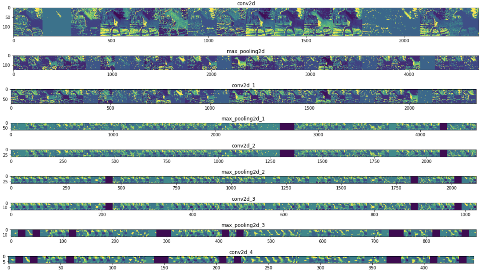
जैसा कि आप देख सकते हैं, आप इमेज के रॉ पिक्सल से बढ़ते हुए ऐब्स्ट्रैक्ट और छोटे प्रज़ेंटेशन तक जाते हैं. प्रज़ेंटेशन, डाउनस्ट्रीम से हाइलाइट होते हैं कि नेटवर्क किस पर ध्यान देता है. साथ ही, ये कम और कम सुविधाएं &चालू हो रहे हैं; ज़्यादातर शून्य पर सेट हैं. वह #33; sparsity कहा जाता है. प्रतिनिधित्व की आज़ादी, डीप लर्निंग की एक अहम सुविधा है.

इससे, इमेज के ओरिजनल पिक्सल के बारे में कम जानकारी मिलती है. हालांकि, इमेज की क्लास के बारे में बेहतर जानकारी मिलती है. आप जानकारी देने वाली पाइपलाइन के तौर पर, CNN (या डीप नेटवर्क) लगा सकते हैं.

11. बधाई हो

आपने #39; सीएनएस का इस्तेमाल करके कॉम्प्लेक्स इमेज को बेहतर बनाना सीखा है. अपने कंप्यूटर के विज़न मॉडल को और बेहतर बनाने का तरीका जानने के लिए, ज़्यादा डेटासेट से बचने के लिए, बड़े डेटासेट के साथ कन्वर्ज़न न्यूरल नेटवर्क (सीएनएन) का इस्तेमाल करें.